This manual describes version 5.12.0 of Qalculate!.
Instructions for the command line calculator can be found in the qalc manual page.
This manual is also available as multiple pages.
Copyright © 2005-2007, 2016-2026 Hanna Knutsson
Feedback
To report a bug or make a suggestion regarding the Qalculate! application or this manual create a new issue at https://github.com/Qalculate/qalculate-gtk/issues.
Table of Contents
- 1. Introduction
- 2. Differences in the “new” Qt user interface
- 3. User Interface
- 4. Expressions
- 5. Calculator Modes
- 6. Propagation of Uncertainty and Interval Arithmetic
- 7. Variables
- 8. Functions
- 9. Units
- 10. Plotting
- A. Function List
- B. Variable List
- C. Unit List
- D. Example expressions
List of Figures
- 3.1. Main Window
- 3.2. Completion
- 3.3. Keypad
- 3.4. Programming keypad
- 3.5. Calculation History
- 3.6. Minimal Window
- 3.7. Variable Manager
- 3.8. Function Manager
- 3.9. Unit Manager
- 3.10. Convert Number Bases Dialog
- 5.1. RPN Mode
- 6.1. Variance Formula
- 7.1. Store Result
- 7.2. New Variable
- 7.3. Matrix/Vector Edit Dialog
- 7.4. Import CSV Dialog
- 8.1. Insert function dialog
- 8.2. Function Edit Dialog
- 8.3. Function Edit Dialog
- 9.1. Unit Conversion View
- 9.2. Unit Edit Dialog (General)
- 9.3. Unit Edit Dialog (Relation)
- 10.1. Plot Data
- 10.2. Plot Settings
- 10.3. Gnuplot
List of Tables
- 3.1. Right Keypad
- 3.2. Left Keypad
- 3.3. Programming Keypad
- 3.4. File Menu
- 3.5. New Menu
- 3.6. Edit Menu
- 3.7. Mode Menu
- 3.8. Functions Menu
- 3.9. Variables Menu
- 3.10. Units Menu
- 3.11. Help Menu
- 4.1. Operators
- 5.1. Supported Number Bases
- B.1. Variables: Basic Constants
- B.2. Variables: Date & Time
- B.3. Variables: Large Numbers
- B.4. Variables: Matrices & Vectors
- B.5. Variables: Atomic and Nuclear Constants
- B.6. Variables: Compton Wavelength
- B.7. Variables: Conversion factors for energy equivalents
- B.8. Variables: Electromagnetic Constants
- B.9. Variables: Particle Mass in MeV*c^(-2)
- B.10. Variables: Particle Mass in kg
- B.11. Variables: Particle Mass in u
- B.12. Variables: Physico-Chemical Constants
- B.13. Variables: Universal Constants
- B.14. Variables: Small Numbers
- B.15. Variables: Special Numbers
- B.16. Variables: Temporary
- B.17. Variables: Traditional Numbers
- B.18. Variables: Unknowns
- B.19. Variables: Utilities
- C.1. Units: Angular Velocity
- C.2. Units: Plane Angle
- C.3. Units: Solid Angle
- C.4. Units: Area
- C.5. Units: Currency
- C.6. Units: Capacitance
- C.7. Units: Electric Charge
- C.8. Units: Electric Conductance
- C.9. Units: Electric Current
- C.10. Units: Electric Dipole Moment
- C.11. Units: Electric Potential
- C.12. Units: Electric Resistance
- C.13. Units: Electrical Elastance
- C.14. Units: Inductance
- C.15. Units: Energy
- C.16. Units: Action
- C.17. Units: Entropy
- C.18. Units: Power
- C.19. Units: Force
- C.20. Units: Dynamic Viscosity
- C.21. Units: Kinematic Viscosity
- C.22. Units: Pressure
- C.23. Units: Information
- C.24. Units: Length
- C.25. Units: Illuminance
- C.26. Units: Luminance
- C.27. Units: Luminous Flux
- C.28. Units: Luminous Intensity
- C.29. Units: Magnetic Field Strength
- C.30. Units: Magnetic Flux
- C.31. Units: Magnetic Flux Density
- C.32. Units: Wave Number
- C.33. Units: Mass
- C.34. Units: Radioactivity
- C.35. Units: Absorbed Dose
- C.36. Units: Dose Equivalent
- C.37. Units: Exposure
- C.38. Units: Ratio
- C.39. Units: Speed
- C.40. Units: Acceleration
- C.41. Units: Substance
- C.42. Units: Catalytic Activity
- C.43. Units: Substance Concentration
- C.44. Units: Temperature
- C.45. Units: Time
- C.46. Units: Frequency
- C.47. Units: Typography
- C.48. Units: Volume
- C.49. Units: Cooking
- C.50. Units: Fuel Economy
- C.51. Units: Imperial Capacity
- C.52. Units: U.S. Capacity
- C.53. Units: Volumetric Flow Rate
Qalculate! is a powerful and highly flexible desktop calculator, but with a comparably simple and minimal user interface.
The center of attention in Qalculate! is the expression entry. Just enter a mathematical expression as you would write it on paper, press Enter, et voilà!
The interpretation of mathematical expressions is flexible and fault tolerant. If you nevertheless enter an expression which is not entirely recognized or is considered ambiguous, Qalculate! will provide an informative, but unobtrusive, error or warning. If an expression cannot be fully solved, Qalculate! will simplify it as far as it can and answer with an expression.
In addition to numbers and arithmetic operators, expressions may contain any combination of variables, units, and functions. These are immediately accessible from the user interface — through automatic completion, or using the menu bar, the object managers, or the calculator keypad.
Qalculate! also provides some specific tools for your convenience, such as a number base conversion dialog and a simple plotting interface.
Although use of Qalculate! for simple calculations should be natural and self-explanatory, reading the rest of the manual can help you maximize your productivity and discover some maybe unexpected features. More advanced users should read on and discover a large number of customization options and the ability to create and modify your own variables, functions and units directly from the user interface.
This manual describes the “classic” GTK version of Qalculate!. Most of it (particularly from chapter 4 and forward) also applies to the “new” Qt version. There are however some significant differences, particularly in the layout of the main window.
In the QT interface the current result is only shown in the history, which is always present below the expression entry. The current result is emphasized with a larger font size, compared to previous results. By default only the parsed expression, and not the entered expression, is displayed in the history.
How the currently edited expression is parsed is either displayed directly in the history or in a tooltip next to the text cursor, instead of below the expression entry. The current result of the expression (calculate-as-you-type) is also displayed in the same way (with a slight delay by default).
The keypad is hidden by default, but can be shown using the second button from the right (the last of the left aligned buttons).
Calculator mode options are changed in the menu opened using the top-left button (above the expression entry). Some settings have been moved to the preferences dialog.
Conversion (including unit conversion) are primarily applied to the current result or expression using the second button from the left.
The contents of the file menu and some of the edit menu in the GTK interface have been moved to the menu accessed using the top-right “hamburger” button.
Table of Contents
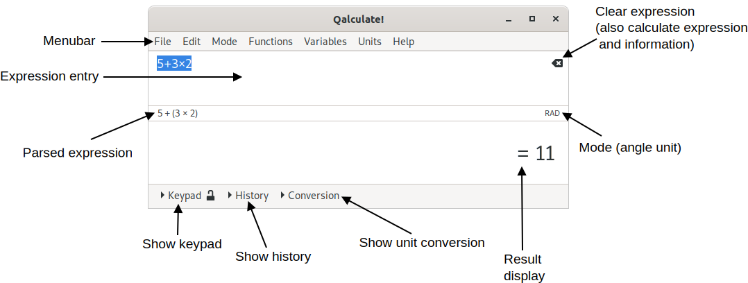
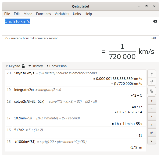
The main window provides a menu bar, the expression entry, the result display and a calculator keypad, history and conversion view (see the section called “Conversion”) which can be shown/hidden by clicking on Keypad, History and Conversion, respectively. When non-default options for the interpretation of expressions have been selected, the choice will be indicated in a small status area below the expression entry, to the right (click to change these choices).
The expression entry is the most important part of the Qalculate! user interface. The normal calculation procedure in Qalculate! is to type in a mathematical expression (e.g. “5 + 5”) and press Enter (or click ). The result (“10”) is then displayed below the expression entry in the result display.
The icon in the upper right corner of the expression entry changes function depending on the current status. While editing the expression an equals sign is shown. When the icon is clicked the expression will be calculated. If this results in an error or a warning, the corresponding icon will be displayed instead, and if this is clicked, or if the pointer is placed over it, the error/warning text will be shown. If no error or warning is triggered, activation of the icon will instead clear the expression entry. No icon is shown when the expression is empty.
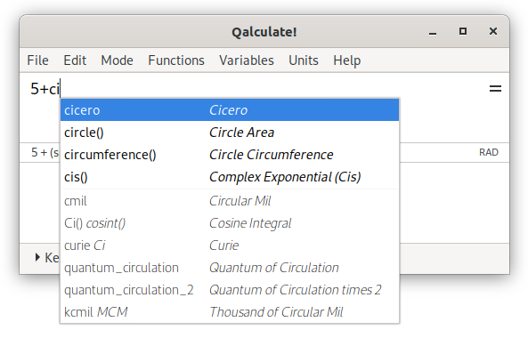
Qalculate! helps out with the expression by giving a list of possible endings to words representing functions, variables and units. Titles, and countries for currencies, will also be searched, but any matches will be placed at the end of the list. The list will narrow with each letter typed. Select an item in the list and the name will be completed. If a function was selected, parenthesis will be added and the position moved for immediate entry of arguments. Completion can be configured from the context menu, or in more detail, from the preferences dialog.
As the expression is typed in, the area directly below the expression entry, to the left, will show useful information. By default the calculator's interpretation of the expression is shown (e.g. “5 × meter” for “5m”). The interpretation will be displayed in red (configurable) if there are errors in the expression or in blue for lesser errors (for example too many arguments in a function). If the last typed-in text represents a function and arguments are about to be entered, the function's name and its arguments will be displayed. The first argument in the information text is highlighted and includes information about its type and restrictions and when an argument has been entered, the next will be highlighted.
After execution of an expression, the whole expression will be marked. This normally means that if something new is entered, the old expression will be overwritten. If, however, an operator (+, −, ×, /, ^) is entered first, the old expression will instead be the target of action. The operator will then apply to the whole expression, which is put in parenthesis. This works on all marked ranges, meaning that this way an expression can conveniently be put in parenthesis. Functions set the selection as their first argument.
The Page Up and Page Down keys will access previously entered expressions. With focus in the expression entry, Page Up traverses backwards in the expression history and Page Down forward. The Up and Down can also be used for the same purpose when the completion list is not shown.
Although the expression entry can display multiple lines of text, the Enter key does not insert a line feed. New lines are automatically created when needed.
The expression entry also accepts commands, preceded be “/”. These commands are the same as in the command line program, qalc.
The font used for the expression entry can be selected in the preferences dialog ( → ).
Right-click in the expression entry to open a context menu, with general text editing options as well as selection of parsing modes (including number base), and menu items which open dialogs for insertion of vectors, matrices, or dates.
The result of calculations is displayed in the open area below the expression entry. The font used for the result display can be selected in the preferences dialog ( → ). Use of Unicode signs can be turned off in the same dialog. Otherwise Qalculate! will try to make the result as fancy as possible and print π for pi, √ for sqrt, € for euro, and so on. Information about customization of the mathematical result output is available in Chapter 5, Calculator Modes.
In front of the result an equals or approximately equals sign is shown. This indicates whether Qalculate! was able to calculate/display the result exact or only approximate, in the current mode.
The result display has a context menu, which pops up when clicking with the right button anywhere in the field. This menu provides a subset of the display alternatives from the mode menu (Table 3.7, “Mode Menu”) and some actions from the edit menu (Table 3.6, “Edit Menu”). See more info in Chapter 5, Calculator Modes.
If you hold the pointer over the result area a tooltip will show the text representation of the result. To make it more obvious what the result means, abbreviations and implicit multiplication are not used here, and excessive parentheses are shown.
To copy the result, either select → , press Ctrl+Alt+C, or copy the text from the history window.
The keypad provides access to a simple traditional number pad and as well as more advanced functionality.
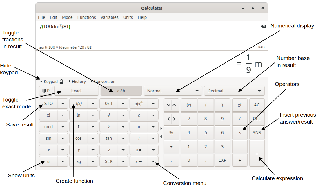
Click on the padlock icon to enable/disable persistent keypad, which makes it possible to display the keypad and the history simultaneously (the keypad view will be independent of the other views).
The top buttons (from left to right) switches between the general keypad and the programming keypad (affects the buttons on the left side, see Table 3.3, “Programming Keypad”), switches between exact and approximate calculation, changes rational number form, selects display mode and selects number base in result (see Chapter 5, Calculator Modes).
The buttons below are separated in two areas. The buttons on the right inserts basic numbers and operators, while most of the buttons to the left inserts or applies mathematical functions to the expression. All buttons on the left is paired with buttons, with downward arrows, that opens a menu with related functionality (generally more mathematical functions).
Most of buttons to the right will do something different depending on which button on the pointing device (mouse) that is clicked (for details see the table below; all actions are displayed as tooltips when holding the pointer over a button). Button press and hold on a button (for approximately half a second) will generally perform the same action as right-click. Right-click or long press on the buttons to the left will open the associated menu.
Selected/marked text in the expression entry is handled in different ways depending on the type of keypad button used. Numbers, variables and units will replace the selected text.
Operators will be placed after any selected text (except bitwise and logical NOT which is placed in front of the selection), which is put in parentheses. This, together with the fact that recently calculated expressions are automatically selected in the entry, means that if you click 5, 9, +, 2, =, × and 2 in order, the result expression is “(59 + 2) × 2”. In RPN mode the operators acts on the top two registers in the stack.
The mathematical functions accessed using keypad buttons (and menus) behave differently depending on the current edited expression. If the cursor is at the end of the expression and there is no operator or parenthesis immediately to left of the cursor (at the end of expression), the whole expression is used as function argument and the expression is immediately calculated using the function (if you type “5 + 2” and then click , “sin(5 + 2)” will be calculated). If text in the expression is selected, the selection will be used as the function argument. If the whole expression was selected the resulting expression will immediately be calculated. Functions that requires more than one argument do not follow these rules and in many cases opens a separate dialog for argument input. In RPN mode the function will always be applied to the register(s) at the top of stack, if the current expression is empty and there are enough registers for functions that require more one argument.
All actions and labels of the buttons on the right can be customized using → (it is also possible to add additional columns of buttons). The default buttons, and associated actions, are listed below.
Table 3.1. Right Keypad
Button | Left-click (button 1) | Right-click (button 3) or long press | Middle-click (button 2) |
|---|---|---|---|
= | Calculates the current expression | MR (memory recall) | MS (memory store) |
ANS | Variable for last calculated value (dynamic) | answer() function (fixed) | - |
DEL | Delete | Backspace | M− (memory minus) |
AC | Clears the expression | MC (memory clear) | - |
+ | Addition operator | M+ (memory plus) | Bitwise AND operator (&) |
− | Subtraction operator | Negate | Bitwise OR operator (|) |
× | Multiplication operator. | Bitwise exclusive OR operator (XOR) | - |
/ | Division operator. | Reciprocal (inv() function) | - |
xy | Exponentiation operator (^) | Square root function (√) | - |
0 | 0 | ⁰ (^0) | ° (degree) |
1 | 1 | ¹ (^1) | Reciprocal (inv() function) |
2 | 2 | ² (^2) | ½ (1/2) |
3 | 3 | ³ (^3) | ⅓ (1/3) |
4 | 4 | ⁴ (^4) | ¼ (1/4) |
5 | 5 | ⁵ (^5) | ⅕ (1/5) |
6 | 6 | ⁶ (^6) | ⅙ (1/6) |
7 | 7 | ⁷ (^7) | ⅐ (1/7) |
8 | 8 | ⁸ (^8) | ⅛ (1/8) |
9 | 9 | ⁹ (^9) | ⅑ (1/9) |
. or , | Decimal point | Blank space | New line |
EXP | E or e (shorthand for 10x) | Exponential function | exp10() function |
) | Right parenthesis. | Right bracket (]) for vectors and matrices | - |
( | Left parenthesis. | Left bracket ([) for vectors and matrices | - |
(x) | Smart parentheses | [] around selection | - |
, or ; | Argument/vector separator | Blank space | New line |
± | Interval/uncertainty operator | Uncertainty function (relative error) | Interval function |
% | Percent (or modulus operator) | Per mille | - |
Left and right arrows | Move cursor one character | Move cursor to beginning or end | - |
Up and down arrows | Cycle through expression history | - | - |
deletes one character to the right or, if the cursor is at the end of the expression, to the left of the cursor (right-click always deletes the character to the left of the cursor). Long press on the button will continuously delete.
inserts the shorthand notation (E or e) for ten raised to the power of x. This only applies to digits (“2E6” equals “2 × 10^6”, “xEy ≠ x × 10^y”). If whole or part of the current expression is selected, “×10^” will instead be inserted after the wrapped selection. If current input base is not 10, than the selected number base will be used as base (e.g. “×16^” for hexadecimal input).
inserts the first answer variable. This variable always contains the last calculated result. This will be updated after each calculation (unlike when using the answer() function with a positive argument).
The “(x)” button (Ctrl+() places opening and closing parentheses around the selected text in the expression entry. If no text is selected either the expression to the right of the cursor (if the cursor is at the beginning of the expression or if there is an operator or left parenthesis to the left of the cursor) or to the left of the cursor is put inside parentheses. If the expression is empty, as well as in some other cases (to avoid broken expression), empty parentheses are inserted.
The arrow buttons works a bit differently than the other. The direction of the action will depend on which half of the button that is pressed (the right side of the button, with the arrow pointing to the right, will move the insert cursor when step forward). Long press on the button will continuously move the cursor (or continuously cycle through the expression history).
The characters used as decimal point and argument separator varies between different locales. The argument separator is used for separation of arguments to functions that takes more than one argument.
Below follows a list of the buttons on the left side (including their menus and associated actions), from left the right, top to bottom.
Table 3.2. Left Keypad
Button | Action | Menu |
|---|---|---|
STO | Stores the current result in a variable. See the section called “Variable creation/editing” | A list of created variables. Left click to insert the variable. Right click for the option to edit or delete the variable, or store the current result in the variable. |
f(x) | Creates a new function. See the section called “Function creation/editing”. | Created and recently used (accessed from this menu, the menubar or the function manager) functions. The last item opens the function manager. |
0xff | Opens the convert number bases dialog. | Bitwise operators |
a(x)b | Factorizes the result (or the current expression). | Expansion of polynomials and expansion of partial fractions, integration and differentiation |
x! | Factorial (e.g. “5!=factorial(5)=5×4×3×2×1=120”) | Other factorial functions and functions related to combinatorics |
ln | Natural logarithm function | Other logarithmic functions |
√ | Square root function | Other root functions |
e | The base of natural logarithms | Exponential and complex exponential functions |
mod | Modulus operator/function | rem(), abs(), gcd() and lcm() functions |
x̄ | Statistical mean function | A selection of statistical functions, and rand() for random number generation |
Σ | Summation function | Π, for() and if() functions |
π | Archimedes' constant (pi) | Pythagoras, Euler's and golden ratio constants, and recently used variables/constants (accessed from this menu, the menubar or the variable manager) and/or a selection of physical constants. The last item opens the variable manager. |
sin | Sine function | sinh(), asin() and asinh() functions, and angle unit selection |
cos | Cosine function | cosh(), acos() and acosh() functions, and angle unit selection |
tan | Tangent function | tanh(), atan() and atanh() functions, and angle unit selection |
i | Imaginary unit (i2 = −1) i | Complex number functions |
z | Unknown variable z | Assumptions for the z variable |
y | Unknown variable y | Assumptions for the y variable |
x | Unknown variable x | Assumptions for the x variable |
x = | Equals operator (primarily used in equations) | Equation solving related functions, and replacement of unknowns in the current result |
u | Opens the unit manager | Recently used units and/or a selection of common units, and a selection of prefixes |
kg | Most recently used unit from the associated menu, or kilogram | All SI base units and SI derived units with special names and symbols, plus litre |
€ (or local currency) | Most recently used unit from the associated menu, or euro/local currency | All current currency units (excludes currencies replaced by euro) |
x ➞ | Convert to operator (selection is unselected). The expression before right arrow or “to” (or the previous result if the expressions begins with “to”) is converted to the unit expression after “to”. See the section called “The “to” (and “where”) operators”. | Convert to base units, optimal unit, or optimal prefix. Below is a list of appropriate units (with common units appended) to convert the current result to. If the result does not include any units options to convert the result to different number bases, fraction and factors appear. The current expression (if modified) is calculated when the menu is opened. |
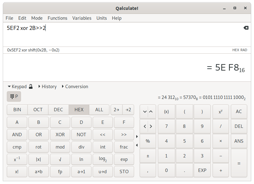
The buttons on the left side can be replaced (using the top left button or Ctrl+P) by a set of buttons for quick access to functions particularly useful for programmers. In place of the menus over the keypad, the current result will be shown in binary, octal, decimal and hexadecimal number bases. The buttons are listed below, from left to right, top to bottom.
Table 3.3. Programming Keypad
Button | Left-click | Right-click or long press |
|---|---|---|
BIN | Switches to binary number base for expressions and result display. | Toggles binary number base for result display on/off. |
OCT | Switches to octal number base for expressions and result display. | Toggles octal number base for result display on/off. |
DEC | Switches to decimal number base for expressions and result display. | Toggles decimal number base for result display on/off. |
HEX | Switches to hexadecimal number base for expressions and result display. | Toggles hexadecimal number base for result display on/off. |
2→ | Toggles two's complement representation on/off for input of negative numbers. | - |
→2 | Toggles two's complement representation on/off for display of negative numbers. | - |
A | Hexadecimal digit | - |
B | Hexadecimal digit | - |
C | Hexadecimal digit | - |
D | Hexadecimal digit | - |
E | Hexadecimal digit | - |
F | Hexadecimal digit | - |
AND | Bitwise AND operator (&) | Logical AND operator (&&) |
OR | Bitwise OR operator (|) | Logical OR operator (||) |
XOR | Bitwise exclusive OR operator (xor) | - |
NOT | Bitwise NOT operator (~) | Logical NOT operator (!) |
<< | Bitwise left shift operator | - |
>> | Bitwise right shift operator | - |
cmp | Bitwise complement (NOT) function (specify bit width and signedness) | - |
rot | Bitwise rotation function | - |
mod | Modulus operator | Remainder operator |
div | Integer division operator | - |
int | Integer part function (“int(-5.2) = -5”) | - |
frac | Fractional part function (“frac(-5.2) = -0.2”) | - |
x-1 | Reciprocal (1/x) function | - |
|x| | Absolute value function (“abs(-5) = 5”) | - |
√ | Square root function | Cube root function |
ln | Natural logarithm function | - |
log2 | Base-2 logarithm function | Base-10 logarithm function |
exp | Exponential function (ex) | Base-2 exponential function (2x) |
x! | Factorial (e.g. “5!=factorial(5)=5×4×3×2×1=120”) | - |
a×b | (Integer) factorizes the result (or the current expression). | - |
fp | Opens a window for conversion between decimal values and floating point formats. | - |
a→1 | code() function (returns numeric code of Unicode character) | char() function (for conversion of numeric code to Unicode character) |
u→d | Function for conversion of Unix timestamp to date and time | Function for conversion of date and time to Unix timestamp |
STO | Stores the current result in a variable. See the section called “Variable creation/editing” | Opens a menu with a list of created variables. Left click to insert the variable. Right click for the option to edit or delete the variable, or store the current result in the variable. |
The history view provides access to previous calculation results (50 rows are reloaded on restart). Previous expressions and results, as well as errors and warnings, are listed. The text of one or multiple entries can be copied to the clipboard using the button to the right of the list.
Double click an item in the history list or use the or the button to paste the selected value or expression into the expression entry. The button inserts the actual value, using the answer() and expression() functions (for results and parsed expressions, respectively) with the current history index (indicated in the left column of the list), as argument, instead of the text (which might be inexact and is not guaranteed to be parsed correctly). This is not possible for the history entries of previous sessions. When an item is double clicked the actual value is used for results, but the text for expressions, allowing editing of the expression.
To the right of the list are also buttons for mathematical operations. These act on the selected history items (the will calculate the sum of the selected values, while the will calculated the difference between the first, uppermost, selected value and the rest, in order). If no value is marked the sign for the operator will be inserted into the expression entry (as the buttons on the keypad). If only one item is selected the buttons also use the current expression (the button will append “+ [value]” to the current expression). The square root button will however only act on single values. When persistent keypad is active, the corresponding buttons on the right side of the keypad provide the same functionality.
Additional actions are available in the context menu of the history list. This includes options to copy the full text of one or multiple entries, search the history, delete or move entries, to clear the whole list, and to bookmark and/or protect entries from deletion when the list becomes too long or is cleared.
It is possible to minimize the footprint of the calculator window using → or Ctrl+Space. This will hide everything but the expression entry and the equals button. The window is expanded to reveal to result, but the result display stays hidden while empty. Restore the window using the keyboard shortcut or the icon in lower right corner of the expression entry.

The menus in the menu bar provides access to most of the functionality of Qalculate!. Their contents are listed and described below.
Table 3.4. File Menu
Menu Item | Description |
|---|---|
New | Submenu for creation of new objects. See Table 3.5, “New Menu”. |
Import CSV File... | Opens a dialog for import of a data file as a matrix or vectors. |
Export CSV File... | Opens a dialog for export of a matrix or vector to a data file. |
Store Result... (Ctrl+S) | Stores the current result as a variable. See the section called “Variable creation/editing”. |
Save Result Image... | Saves the result display to a PNG image. |
Save Definitions | Saves all user definitions (variables, functions and units). |
Update Exchange Rates | Downloads current exchange rates from the Internet. |
Plot Functions/Data | Opens the plot dialog. See Chapter 10, Plotting. |
Convert Number Bases (Ctrl+B) | Opens the number bases converter. See the section called “Convert Number Bases Dialog”. |
Floating Point Conversion (IEEE 754) | Opens a window for conversion between decimal values and floating point formats. |
Calendar Conversion | Opens a window for conversion of dates between different calendars. |
Percentage Calculation Tool | Opens a window for quick and easy percentage calculation. |
Periodic Table | Shows a periodic table, with property values which can be inserted in the expression, in a new window. |
Minimal Window (Ctrl+Space) | Hides everything but the expression entry, the result (when not empty), and the equals button. |
Quit (Ctrl+Q) | Exits Qalculate! |
Table 3.5. New Menu
Menu Item | Description |
|---|---|
Variable | Opens the variable edit dialog for creation of a new variable. |
Matrix | Opens a dialog for entry of a new matrix variable. |
Vector | Opens a dialog for entry of a new vector variable. |
Unknown Variable | Opens the variable edit dialog for creation of a new unknown variable. |
Function | Opens the function edit dialog for creation of a new function. |
Data Set | Opens the data set edit dialog for creation of a new data set. |
Unit | Opens the unit edit dialog for creation of a new unit. |
Table 3.6. Edit Menu
Menu Item | Description |
|---|---|
Variables (Ctrl+M) | Opens the variable manager. See the section called “Variable/Function/Unit Managers”. |
Functions (Ctrl+F) | Opens the function manager. See the section called “Variable/Function/Unit Managers”. |
Units (Ctrl+U) | Opens the unit manager. See the section called “Variable/Function/Unit Managers”. |
Data Sets | Opens the data set manager. |
Factorize | Factorizes the current result. For multivariate rational polynomials, only square free factorization is fully supported. |
Expand | Expands the current result. |
Expand Partial Fractions | Applies partial fraction decomposition to the current result. |
Set Unknowns... | Opens a dialog where the values of unknown variables in the result can be set and the result recalculated. |
Convert To Unit | Submenu with units. Select a unit to convert the current result. |
Set Prefix | Submenu for choice of unit prefix in current result. |
Convert To Unit Expression (Ctrl+T) | Opens the convert to unit view for conversion of result to custom unit expression. See the section called “Conversion”. |
Convert To Base Units | Splits up unit(s) in the current result into base units. |
Convert To Optimal Unit | Tries to convert the units in the current result to as few units and exponents as possible. Only SI units are used for the conversion, but if no improvement is achieved, the original units are kept. Currencies are converted to the local currency, unless deactivated in the preferences dialog. |
Convert To Optimal SI Unit | Tries to convert the units in the current result to as few units and exponents as possible. Non-SI units are not kept, even if the number of units increases, and the automatic alternative is prioritized. Currencies are converted to the local currency, unless deactivated in the preferences dialog. |
Insert Date | Opens a dialog for date selection (for insertion in the current expression). |
Insert Matrix | Opens a dialog where you can create a matrix in a spreadsheet-like table and insert into the expression entry. If selected expression text is a matrix, then the matrix is edited. |
Insert Vector | Opens a dialog where you can create a vector in a spreadsheet-like table and insert into the expression entry. If selected expression text is a vector, then the vector is edited. |
Copy Result (Ctrl+Alt+C) | Copies the current result to the clipboard. |
Copy Result as Unformatted ASCII | Copies the current result with formatting removed and Unicode symbols replaced with corresponding ASCII characters. |
Keyboard Shortcuts | Opens a dialog for editing key bindings. |
Customize Keypad Buttons | Opens a dialog for customizing the labels and actions for the keypad buttons on the right side, and optionally adding additional columns of buttons. |
Preferences | Opens the preferences dialog, which controls settings for visual appearance and start/exit actions. |
Open Settings Folders | Opens the folder(s) containing the configuration files in the default file manager. |
Table 3.7. Mode Menu
Menu Item | Description |
|---|---|
Number Base | Submenu with a list of number bases (binary, octal, decimal, duodecimal, hexadecimal, sexagesimal, time format, and other bases, and roman numerals) to select for result display, and a menu item (Ctrl+B) for opening a dialog to switch number bases in expression (input) and result (output). |
Numerical Display | Submenu which selects numerical display mode. See Chapter 5, Calculator Modes. |
Rational Number Form | Submenu which switches between display of rational numbers as fractions or decimal numbers. See Chapter 5, Calculator Modes. |
Interval Display | Submenu with options that determines how intervals and results with associated uncertainty are shown. The adaptive option is the same as significant digits display unless an interval has been explicitly specified in the expression. |
Unit Display | Submenu which controls the display of units and prefixes. See Chapter 5, Calculator Modes. |
Abbreviate Names | Toggles on/off use of abbreviation for unit, prefix, variable and function names in result display. |
Enabled Objects | Submenu which enables/disables variables, functions, units and unknowns (will not affect defined unknown variables and quoted unknowns), calculation of variables (if calculation of variables is not on, all variables will be treated as unknown), and units in variables for physical constants. Here you can also disable complex and infinite results. |
Approximation | Submenu which switches between different approximation modes. |
Interval Calculation | Submenu for selection of algorithm for interval calculation / uncertainty propagation. |
Angle Unit | Submenu which sets the default angle unit for trigonometric functions. |
Assumptions | Submenu which changes default assumptions for unknown variables. |
Algebraic Mode | Submenu with options to automatically expand or factorize the final result. In this menu, the option toggle on/off use of the assumption that unknown denominators not are zero is also found. This alternative makes it possible to avoid the situation where expressions such as “(x-1)/(x-1)” can not be further simplified because the denominator might be zero (if x equals 1). |
Parsing Mode | Submenu with options to control how expressions are parsed (read/interpreted). There are three main modes to choose from. In addition the “read precision” option enables/disables interpretation of input numbers with decimals as approximations with a precision equal to the number of digits (after preceding zeroes), and “limit implicit multiplication” limits the use of implicit multiplication for parsing and display of expressions. For more information see the section called “Implicit Multiplication and Parsing Modes”. Additionally RPN and chain syntax modes can be selected. |
Precision | Opens a dialog to change precision in calculations. |
Decimals | Opens a dialog to change displayed number of decimals. |
Calculate As You Type | When activated the current expression will be continuously calculated on each single change. |
Chain Mode | (De)activates chain mode. In chain mode the expression are, when operators are entered, transformed to mimic the behavior of traditional simple calculators in immediate execution mode. The result is equivalent to that of the chain syntax (see the section called “Implicit Multiplication and Parsing Modes”). The result is updated each time an operator is entered. |
RPN Mode (Ctrl+R) | (De)activates the Reverse Polish Notation stack (not RPN syntax). For details see the section called “The RPN Mode” |
Meta Modes | Provides a list of available meta modes for loading and menu items to save and delete modes. |
Save Default Mode | Saves the current calculator mode as the startup default. |
Table 3.8. Functions Menu
Menu Item | Description |
|---|---|
(Recent functions list) | Select a function to open the insert function dialog. |
(Function list) | Select a function to open the insert function dialog. |
Table 3.9. Variables Menu
Menu Item | Description |
|---|---|
(Recent variables list) | Select a variable to insert it into the expression entry. |
(Variable list) | Select a variable to insert it into the expression entry. |
Table 3.10. Units Menu
Menu Item | Description |
|---|---|
(Recent units list) | Select a unit to insert it into the expression entry. |
(Unit list) | Select a unit to insert it into the expression entry. |
Table 3.11. Help Menu
Menu Item | Description |
|---|---|
Contents (F1) | Opens this help. |
Report a Bug | Opens the web interface for creation of bug reports. |
Check for Updates | Checks if a new version of Qalculate! is available. |
About | Info about Qalculate! |
The variables, functions, and units windows provide a structural way of working with variables, functions and units (collectively referred to as objects). The windows for the three different objects are essentially similar. They can be opened from the edit menu, or using Ctrl+M, Ctrl+F and Ctrl+U for variables, functions and units respectively.
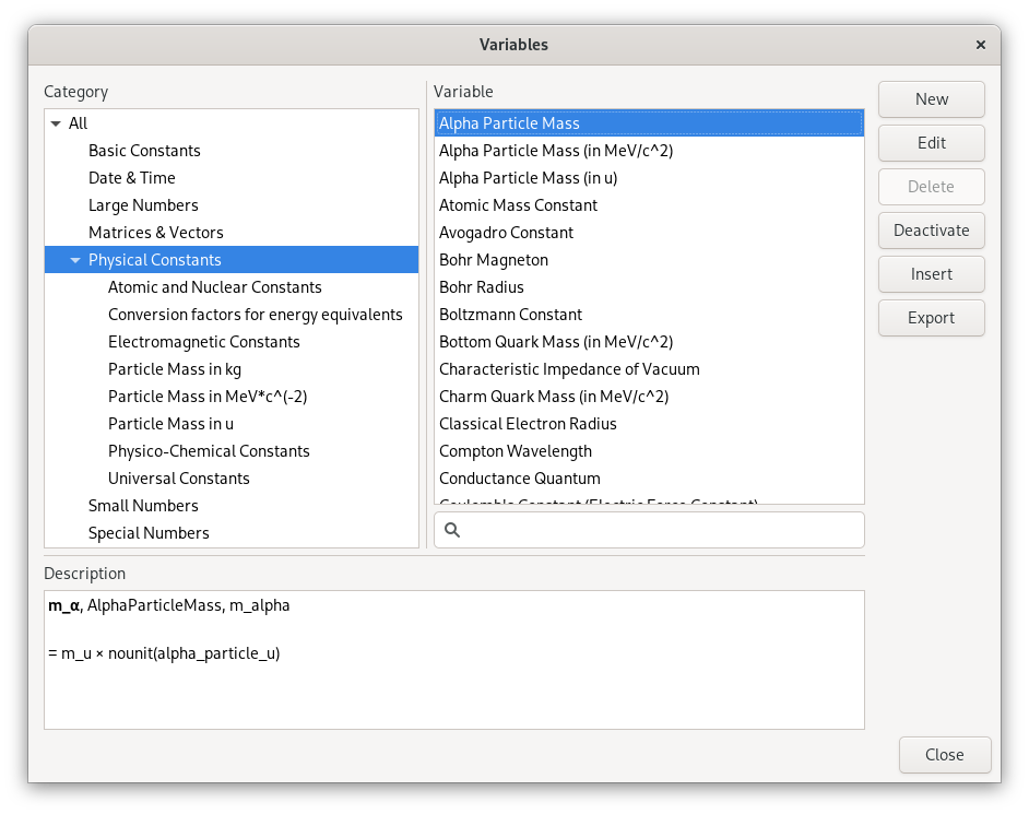
To the left is a category tree and beside that is a list of all objects in the selected category, including all subcategories. Objects without a category are put under “Uncategorized”. Objects created by the user can also be found under the category “User variables”, “User functions”, and “User units”, shown at the top of the list. Deactivated objects are only found in the “Inactive” top category. Below the categories and objects lists, a description of the selected object is shown.
The buttons on the right work on the selected object in the list. opens a dialog for creation of a new object, while opens the same dialog to edit the selected unit. removes the object and toggles recognition in expressions on/off. in the variables and units windows adds the object to the current expression, while in the functions window opens a dialog for entering arguments and provides options for insertion of the function or direct calculation. The unit manager provide an additional button for conversion of the current result, the variable manager a button for export to a data file, and the function manager a button for applying functions with a single argument directly to the current expression.
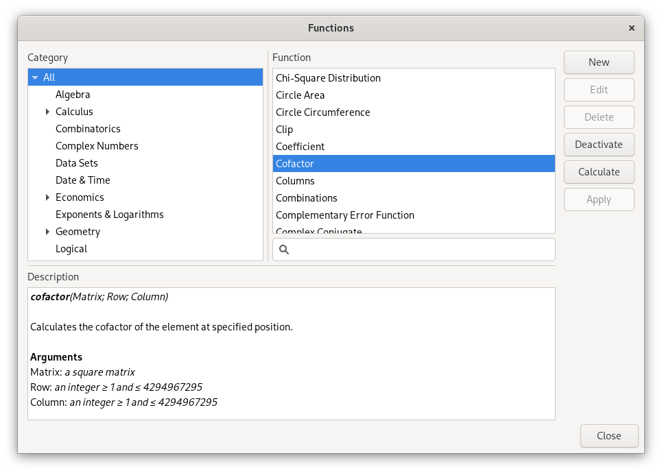
The function manager has a description box at the bottom, which shows the syntax, description and arguments of the selected function.
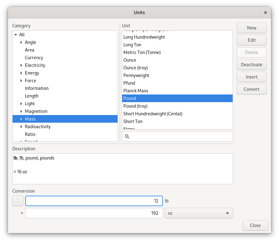
The unit manager has an area for quick conversion between units. This converts between the selected unit in the list and the selected unit in the menu. Both the menu and the list filters the units as you type. Units are converted by specification of a quantity, in the entry next to the unit to convert from, followed by Enter.
For more information about variables, functions and units, see Chapter 7, Variables, Chapter 8, Functions and Chapter 9, Units.
The number bases dialog, accessible from the , is an efficient and convenient tool for conversion between binary, octal, decimal, duodecimal, hexadecimal and Roman numbers. This dialog contains entries for each number base. When a number is typed in any of the entries, the others are automatically updated to display the current number in their format. Numbers, or expressions, entered follow the same rules as expressions in the main expression entry.
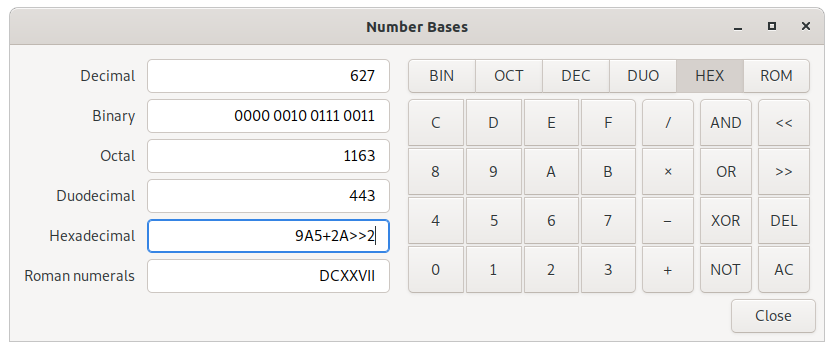
Table of Contents
Expressions are mathematical statements. Mathematical questions are asked through expressions, which contains objects tied together with operators. The result of an expression may also be an expression, if the result is not a single object. Apples and oranges can be mixed, but the result will hold them apart. Qalculate! knows algebra.
In Qalculate! mathematical entities, such as numbers and variables, are referred to as objects. The recognized object types are listed below.
- Numbers
These are the regular numbers composed by digits 0-9 and a decimal sign — a dot, or a comma if it is the default decimal point in the locale/language used. If comma is used as decimal sign, the dot is still kept as an alternative decimal sign, if not explicitly turned off in the preferences dialog with (to allow it to be used as thousand separator instead). Numbers include integers, real numbers, and complex numbers. The imaginary part of complex numbers is written as a regular number followed by the special variable “i” (can be changed to a “j”, placed in front of the imaginary part, in the preferences dialog), which represents the square root of -1 (e.g. “2 + 3i”). Spaces between digits are ignored (“5 5 = 55”). “E” (or “e”) can be considered as a shortcut for writing many zeroes and is equivalent to multiplication by 10 raised to the power of the right-hand value (e.g. “5E3 = 5000”).
Sexagesimal numbers (and time) can be entered directly using colons (e.g. “5:30 = 5.5”). A number immediately preceded by “0b”, “0o”, “0d” or “0x” is interpreted as a number with base 2, 8, 12 or 16, respectively (if the default base is 10, e.g. “0x3f = 63”). The number base can also be selected, either by using the base(), bin(), oct(), hex() and roman() functions, or by setting the base used for all numbers in the whole expression from → → . For details about supported number bases see Table 5.1, “Supported Number Bases”.
- Intervals
A number interval can be entered using the interval() function (specifies the upper and lower limit of the interval), the uncertainty() function (specifies relative or absolute uncertainty), or using “±” or “+/-”, specifying the width of the interval after the mid value (e.g. “5±1 = uncertainty(5, 1, 0) = 5±20% = uncertainty(5, 0.2) = interval(4, 6)”. If activated, concise notation can also be used, e.g. “1.2345(67) = 1.2345±0.0067”. If the read precision option is activated, decimal numbers are interpreted as an interval between the numbers that are normally rounded to the entered number (e.g. “1.1 = 1.1±0.05”). If interval calculation using variance formula is activated (default), the interval represents the standard uncertainty (deviation) of the value.
- Vectors and Matrices
A matrix is a two-dimensional rectangular array of mathematical objects. Vectors are matrices with only one row or column, and thus one-dimensional sequences of objects. Vectors and matrices are generated by vector(), matrix() and similar functions, or using a syntax in the form of “[1 2 3 4]” and “[1 2; 3 4]”, with columns separated by space or comma and rows separated by semi-colon, or “(1, 2, 3, 4)” and “((1, 2), (3, 4))”. Vectors with a sequence of numbers can be input using “...” (e.g. “1...4”), or colon (e.g. “[1:4]”, or “[1:1:4]” where the second value specifies the increment). Vectors are generally considered as matrices with one row (row vector) in operations that expect a matrix (e.g. matrix multiplication).
Matrices and vectors with many elements are easier to handle if stored in variables. A single element of a vector variable can be selected using the element() function, or by placing the index (first index is 1) in parenthesis, e.g. “v(2)” or “v[2]” (the latter syntax can also be used for vector returning functions).
- Variables/Constants
See Chapter 7, Variables.
- Functions
See Chapter 8, Functions.
- Units and Prefixes
Qalculate! understands abbreviated, plural and singular forms of unit names and prefixes. Prefixes must be put immediately before the unit to be interpreted as prefixes — “5 mm = 0.005 m”, but “5 m m = 5 m^2”. Also, for convenience units allow the power operator to be left out. A number following immediately after a unit is interpreted as an exponent (e.g. “5 m2 = 5 m^2”). This does not apply to currencies, as they might be put in front of the quantity. More information in Chapter 9, Units.
- Unknowns
Unknowns are text strings without any associated value. These are temporary unknown variables with default assumptions. Unknowns can also be explicitly entered by placing a backslash (“\”) before a single character (e.g. “5\a + 2\b”) or using quotation marks (“"” or “'”) before and after a text string (e.g. “5 "apples" + 2 "bananas"”). If unknowns are activated (+ → ) and Qalculate! finds a character that are not associated with any variable, function or unit in an expression, then it will be regarded as an unknown variable. See Chapter 7, Variables.
- Date and Time
Date/time values are specified using quoted text string (quotation marks are not needed for function arguments), using standard date and time format (YYYY-MM-DDTHH:MM:SS). Some local formats are also supported, but not recommended. The local time zone is used, unless a time zone is specified at the end of the time string (Z/UTC/GMT or +/-HH:MM). Date/time supports a small subset of arithmetic operations. The time units represents calendar time, instead of average values, when added or subtracted to a date.
- Text
This category represent a number of different function argument types, such as regular text and file names. They can, but do not need to be put in quotes except when containing the argument separator (“,” or “;”).
- Comments
All text after a hashtag (e.g. “(5×2)/2 #calculating triangle area”) is treated as a comment, which are added to the history. Use double hashtags (“##”) at the beginning of the expression to add a comment as a separate history item at the top.
To avoid confusion, functions, units, variables and unknown variables can independently be disabled.
Variables, functions and units are all accessible in the menus and in the variable, function and unit managers, If their names are not remembered. Functions accessed this way have some extra conveniences. If the function has at least one argument, a dialog will pop up where arguments can be entered and a description of the function and its arguments is available.
Qalculate! can handle most commonly used symbols for certain variables, functions and units, even though most are difficult to find on a keyboard. These include π for pi, √ for sqrt, € for euro, and so on. Most importantly it is possible to copy these symbols when used in the result.
For more information about variables, functions and units, see Chapter 7, Variables, Chapter 8, Functions and Chapter 9, Units.
The following operators are defined in Qalculate! and may be used in expressions. Word operators (such as AND) must be surrounded by space (e.g. “5 mod 2”, not “5mod2”.
Table 4.1. Operators
Operation | Symbol | Description | Example | Result |
|---|---|---|---|---|
Addition | +, plus | Adds the right value to the left value. | 1 + 1 | 2 |
Subtraction | −, minus | Subtracts the right value from the left value. | 1 − 1 | 0 |
Multiplication | ×, ⋅, *, times | Multiplies the left value by the right value. | 2 × 2 | 4 |
Division | /, per | Divides the left value by the right value. | 2 / 2 | 1 |
Remainder | %, rem | Returns the remainder after (truncated) division. The result will have the same sign as the dividend. | 3%2 | 1 |
Modulo | %%, mod | Returns the remainder after (floored) division. The result will have the same sign as the divisor. | 3 mod -2 | -1 |
Integer Division | //, \, div | Divides the left value by the right value and rounds the result towards zero. | 5 // 2 | 2 |
Exponentiation | ^, ** | Raises the left value by the right value. Can also be typed as “**”. Note that x^y^z equals x^(y^z), and not (x^y)^z. Note also that for non-integer exponents with negative bases, the principal root is returned and not the real root (“(-8)^(1/3)” equals “1 + 1.73i” instead of -2). To calculate the real root for negative values, use the cbrt() and root() functions. | 2^3 | 8 |
10^x | E | Multiplies the left value with 10 raised to the power of the right value. Equivalent to the exponential number format in result display. E is as much an operator as part of numbers. | 1E3 | 1000 |
Factorial | ! | Returns the factorial of the value to the left of the operator. If the operator is repeated the corresponding multifactorial is returned. | 5! | 120 |
Parenthesis | ( and ) | Evaluates the expression in parenthesis first. | 5 × (1 + 1) | 10 |
Parallel sum | ∥, || | Returns the reciprocal value of a sum of reciprocal values. || is interpreted as parallel if units are used, otherwise as logical OR. | 10 Ω || 6 Ω | 3.75 Ω |
Equals | = | Returns true if the left value equals the right value. Unknown variables (e.g. x) are isolated if the expression does not evaluate as true or false. | 1 = 2, 5x = 5 | 1, x=1 |
Not equals | ≠, != | Returns true if the left value does not equals the right value. Unknown variables (e.g. x) are isolated if the expression does not evaluate as true or false. | 1 != 2, x + 2 != 5 | 1, x != 3 |
Less than | < | Returns true if the left value is less than the right value. Unknown variables (e.g. x) are isolated if the expression does not evaluate as true or false. | 1 < 2 | 1 |
Greater than | > | Returns true, if the left value is greater than the right value. Unknown variables (e.g. x) are isolated if the expression does not evaluate as true or false. | 1 >2 | 0 |
Less than or equal | ≤, <= | Returns true if the left value is less than or equal the right value. Unknown variables (e.g. x) are isolated if the expression does not evaluate as true or false. | 1 <= 2 | 1 |
Greater than or equal | ≥, >= | Returns true if the left value is greater than or equal the right value. Unknown variables (e.g. x) are isolated if the expression does not evaluate as true or false. | 1 ≥ 2, x + 5 ≥ 7 | 0, x ≥ 2 |
Logical NOT | !, not | Returns true if the value to the right is false. | !(1>2) | 1 |
Logical OR | ||, or | Returns true if the right or left value is true. | 1>2 || 2>1 | true |
Logical XOR | ⊕, xor | Returns for true if one, but not both, of the right or left value is true. | 1>2 ⊕ 2>1 | true |
Logical NOR | nor | Returns true if both the right and left value is false. | 1>2 nor 2>1 | false |
Logical AND | &&, and | Returns true if both the right and left value is true. | 1>2 && 2>1 | false |
Logical NAND | nand | Returns true if the right or left value is false. | 1>2 nand 2>1 | true |
Bitwise NOT | ¬, ~ | Equivalent to -1 − x. | ~(0010 | 1100) | -1111 |
Bitwise Shift Left | << | Shifts the bits of the left value x steps to the left, where x is the value on the right. Implemented as a shortcut for shift() | 0011 << 1 | 0110 |
Bitwise Shift Right | >> | Shifts the bits of the left value x steps to the right, where x is the value on the right. Implemented as a shortcut for shift() | 0011 << 1 | 0001 |
Bitwise OR | ∨, | | If a bit is 1 in one of the numbers set it to 1, otherwise 0. Also functions as elementwise logical operator on vectors. | 0010 | 1100 | 1110 |
Bitwise XOR | ⊻, ^^, xor | If a bit is 1 in one of the numbers and not in the other, set it to 1, otherwise 0. Can normally also be used as logical XOR. ⊻ can be input using Ctrl+^ (or just ^ if selected in preferences) on the keyboard. | 1010 ⊻ 1100 | 0110 |
Bitwise AND | ∧, & | If a bit is 1 in both numbers set it to 1, otherwise 0. Also functions as elementwise logical operator on vectors. | 1010 & 0011 | 0010 |
Dot Product | ., dot | Returns the dot product for two vectors. | [1, 2, 3].[4, 5, 6] | 32 |
Cross Product | ⨯, cross | Returns the cross product for two vectors. | [1, 2, 3] cross [4, 5, 6] | [-1, 6, -3] |
Elementwise Multiplication | .×, .* | Multiplies each element of a vector/matrix with the corresponding element in another vector/matrix, or a scalar. | [1, 2, 3].*[4, 5, 6] | [4, 10, 18] |
Elementwise Division | ./ | Divides each element of a vector/matrix by the corresponding element in another vector/matrix, or a scalar. | [2, 4, 6]./2 | [1, 2, 3] |
Elementwise Exponentiation | .^ | Raises each element of a vector/matrix by the corresponding element in another vector/matrix, or a scalar. | [1, 2, 3].^2 | [1, 4, 9] |
Transpose | .' | Returns the transpose of the matrix to the left of the operator. | [1 2 3; 3 4 5].' | [1 3; 2 4; 3 5] |
Set Operators | ∪, ∩, ∖, ⊖, | Applies set operation to vectors to the left and right of the operator. | [1, 2, 3]∩[2, 3, 4] | [2, 3] |
Combination | comb | Same as comb() function. | 5 comb 2 | 10 |
Permutations | perm | Same as perm() function. | 5 perm 2 | 20 |
Save as Variable/Function | :=, = | Saves the value or expression to the right of the operator as a variable or function (as save() function). If colon is omitted, the expression is calculated before it is assigned to the variable. | var1:=5 func1():=x+y var1=ln(5)+2 |
The multiplication sign can generally be left out. This is not true for numbers (“5(5) = 25” but “5 5 = 55”). Expressions can also generally be written with or without spaces with the same result (“2xsin(2)” equals “2 x sin(2)” which equals “2 × x × sin(2)”), but be careful. The vast number of functions and units means that without separating spaces, the result might not be obvious. To avoid confusion Qalculate! can limit the use of implicit multiplication ( → ), so that space, operator or parenthesis must be put between functions, units and variables (in this mode “esqrt(5)” does not equal “e × sqrt(5)”). Also note that unit prefixes must be put immediately before the unit, to be interpreted as prefixes (“5 mm = 0.005 m”, but “5 m m = 5m^2”). You can see how the expression was interpreted in the history window.
Usually, mathematical expressions are written as normally expected. Standard operator precedence apply. Expressions are evaluated according to the following priorities:
Parenthesis
E (10^x)
Exponentiation (^, .^)
Functions (e.g. “sqrt(2)”)
Bitwise NOT (~)
Logical NOT (!)
Multiplication, division, integer division, remainder, modulo (*, /, //, %, %%, .*, ./, ., ⨯)
Parallel sum (∥)
Addition and subtraction (+, −)
Bitwise NOT (~)
Bitwise Shift (<<, >>)
Comparison (>, <, =, >=, <=)
Bitwise AND (&)
Bitwise XOR (⊻)
Bitwise OR (|)
Logical AND (&&)
Logical NAND
Logical NOR
Logical OR (||)
Logical XOR (⊕)
The evaluation of short/implicit multiplication, without any multiplication sign (e.g. “5x”, “5(2+3)”), differs depending on the parsing mode. In the conventional mode implicit multiplication does not differ from explicit multiplication (“12/2(1+2) = 12/2×3 = 18”, “5x/5y = 5 × x/5 × y = xy”). In the “parse implicit multiplication first” mode, implicit multiplication is parsed before explicit multiplication (“12/2(1+2) = 12/(2 × 3) = 2”, “5x/5y = (5 × x)/(5 × y) = x/y”). The default adaptive mode works as the “parse implicit multiplication first” mode, unless spaces are found (“1/5x = 1/(5 × x)”, but “1/5 x = (1/5) × x”). In the adaptive mode unit expressions are parsed separately (“5 m/5 m/s = (5 × m)/(5 × (m/s)) = 1 s”). Function arguments without parentheses are an exception, where implicit multiplication in front of variables and units is parsed first regardless of mode (“sqrt 2x = sqrt(2x)”).
If the limit implicit multiplication option is activated, the use of implicit multiplication when parsing expressions and displaying results will be limited to avoid confusion. For example, if this mode is not activated and “integrte(5x)” is accidently typed instead of “integrate(5x)”, the expression is interpreted as “int(e × e × (5 × x) × gr × t)” (displayed in history window). The result will then without any error be “int(2.3940139x × km^2)” instead of “2.5x^2”. If limit implicit multiplication is activated, the mistyped expression would instead show an error telling that “integrte” is not a valid variable, function or unit (unless unknowns is enabled in which case the result will be “5 "integrate" × x”). When implicit multiplication is limited, variables, functions and units must be separated by a space, operator or parenthesis (“xy” does not equal “x × y”).
In addition there are two special parsing modes — RPN syntax (for details see the section called “The RPN Mode”) and chain syntax. The chain syntax interprets expressions in a manner similar to the immediate execution mode of a traditional calculator. Instead of using the standard order of operations, the expression is simply calculated from left to right (e.g. “1 + 2 × 3 = (1 + 2) × 3 = 9” instead of “1 + 2 × 3 = 1 + (2 × 3) = 7”). Functions, with a single argument, apply to the value immediate to the left of the function name (e.g. “1 + 2 sin = 1 + sin(2)”), unless parentheses are used.
Putting “ to ” (or a right arrow, e.g. “->” but not “>”) followed by an expression at the end of the mathematical expression is mainly used for unit conversion (see the section called “Conversion”). There are however also some convenient commands that can be typed after “ to ”. Here is a list of possible “to” values:
- A unit or unit expression
Convert to a unit or a unit expression (e.g. “5 ft + 2 in to meter = 1.5748 m” or “50 mph to km/h ≈ 80 km/h”). Prepend with a question mark (?) to request the optimal prefix. Modifiers in front of the question mark selects the type of prefixes used — 'b' for binary prefixes, 'd' for decimal prefixes, and 'a' for all decimal prefixes including centi, deci, etc. (e.g. “8 × 1024 bits to b?bytes = 1 kibibyte”). Prepend with + or - to force/disable use of mixed units (e.g. “5 m to + ft ≈ 5 yd + 1 ft + 4.9 in”).
- A physical constant or a variable
Convert to variable as unit (e.g. “500 km/ms to c ≈ 1.7 c”).
- base
Convert to base units (e.g. “1 lux to base = 1 cd/m2”).
- optimal
Convert to optimal unit (e.g. “(10 J)/(2 s) to optimal = 5 W”).
- prefix
Convert to optimal prefix (e.g. “€5000 to prefix = k€5”).
- mixed
Convert to mixed units (e.g. “90 s to mixed = 1 min + 30 s”.
- bin, binary
Show as binary number (e.g. “sqrt(900) to bin = 0001 1110”). Append an integer to specify the number of bits (e.g. “4 to bin16 = 0000 0000 0000 0100”).
- oct, octal
Show as octal number (e.g. “52 to octal = 64”).
- duo, duodecimal
Show as duodecimal number (e.g. “152 to duo = 108”).
- hex, hexadecimal
Show as hexadecimal number (e.g. “623 to hex = 026F”). Append an integer to specify the number of bits (e.g. “4 to hex16 = 0004”).
- sexa, sexa2, sexa3, sexagesimal
Show as sexagesimal number (e.g. “7.33 to sexagesimal = 7°19′48″”). For sexa2, arcseconds are hidden, and for sexa3 arcseconds are rounded.
- longitude, longitude2, latitude, latitude2
Show as sexagesimal latitude/longitude (e.g. “-7.33 to latitude = 7°19′48″S”). longitude2/latitude2 only shows degrees and arcminutes (e.g. “-7.33 to latitude2 = 7°19.8′S”).
- bijective
Show as bijective base-26 number (e.g. “731 to bijective = ABC”).
- binary16 / fp16, binary32 / float / fp32, binary64 / double / fp64, fp80, binary128 / fp128
Show as binary representation of IEEE 754 16-bit (half precision), 32-bit (single precision), 64-bit (double precision), 80-bit (x86 extended format), or 128-bit (quadruple precision) floating-point number.
- time
Show in time format (e.g. “7.25 to time = 7:15”.
- roman
Show as Roman numerals (e.g. “1984 to roman = MCMLXXXIV”).
- Unicode
Show as Unicode character(s) (uses UTF-32 for conversion, e.g. “0x178 to Unicode = Ÿ”).
- base #
Show using the specified base (e.g. “523 to base 20 = 163” or “circumference(1) to base pi = 20”).
- bases
Show as binary, octal, decimal, duodecimal, hexadecimal and Roman number (opens convert bases dialog with the mathematical expression).
- rectangular, cartesian
Show complex number in rectangular form (e.g. “0.28i − 2 to complex = 0.28i − 2”).
- exponential
Show complex number in exponential form (e.g. “0.28i − 2 to exponential ≈ 2e^(3i)”).
- polar
Show complex number in polar form (e.g. “0.28i − 2 to polar ≈ 2(cos(3) + i × sin(3))”).
- angle, phasor
Show complex number in angle/phasor notation (e.g. “0.28i − 2 to angle ≈ 2∠3”).
- cis
Show complex number in cis form (e.g. “0.28i − 2 to angle ≈ 2 cis 3”).
- fraction, 1/n
Show as mixed or simple (prepend with “-”) fraction (“1.25 to fraction = 1 + 1/4”).
- 1/#
Show as mixed or simple (prepend with “-”) fraction with a specific denominator (“2.7 to 1/3 ≈ 2 + 2/3”, “2.7 to -1/3 ≈ 8/3”).
- sci, scientific
Show with scientific notation (“123456 to sci = 1.234 56 × 105”
- eng, engineering
Show with engineering notation (“1011 to eng = 100 × 109”
- simple
Show with non-scientific notation (“1015 to simple = 1 000 000 000 000 000”
- partial fraction
Show expanded partial fractions (e.g. “1 / (x2 + 2x − 3) to partial fraction = 1 ∕ (4x − 4) − 1 ∕ (4x + 12)”).
- factors
Show factorized (algebraic or integer factorization, e.g. “3 645 678 to factors = 857 × 709 × 3 × 2” or “x2 + 4x + 4 to factors = (x + 2)2”).
- calendars
Show date in different calendars (opens calendar conversion dialog).
- UTC
Show date and time using UTC time zone.
- UTC+/-hh[:mm]
Show date and time using specified time zone (e.g. UTC+08).
If “to” is not preceded by an expression, the previous result will be converted.
Similarly “where” (or alternatively “/.”) can be used at the end (but before “to”), for variable assignments, function replacements, etc. (e.g. “x+y where x=1 and y=2”, “x^2=4 where x>0”, and “sin(5) where sin()=cos()”). Variables assignments can also be placed before the expression, separated by comma, e.g. “x=1, y=2, x+y”, but this syntax is more strict.
Note that “to” and “where” can only be applied to the whole expression. Everything before the operator is always treated as the expression to convert (or apply replacement to), and everything after as the conversion/replacement expression, regardless of any parentheses.
Table of Contents
Qalculate! provides flexible parsing, calculation output and result display. There are several ways in which parsing of expression and display of results can be customized. These modes can generally be changed through the mode menu. The state of each mode can be saved under a name in → for quick access. The Preset and Default meta modes are always available and represents the state when Qalculate! is load for the first time and the mode settings automatically loaded at each startup (and by default saved on exit), respectively. Different modes are summarized below.
- Number Bases
Non-decimal bases can be selected for display of numbers in the result and parsing of numbers in expressions. This include regular number bases (binary, octal, hexadecimal, sexagesimal) as well as sexagesimal time format and roman numerals. Other number bases, as well as base for expression input, can be selected from a dialog window accessed from → → or → → .
Table 5.1. Supported Number Bases
Radix
Digits
Comments
2-10
1-10
12
1-10, ↊/X/A/a, ↋/E/B/b
Supports all functions, variables and units that do not conflict with digits.
11-36
1-10, A-Z (case insensitive)
Supports all functions, variables and units that do not conflict with digits.
37-62
1-10, A-Z, a-z
Supports all functions, variables and units that do not conflict with digits.
> 62
Unicode characters (“0” = 62) or escaped values (“\523” = 523, “\x7f” = 127)
Does not support operators, functions, variables or units. Result display only uses escaped values except for with base 1114112 (the “Unicode” base).
Negative bases (e.g. -2)
Same as corresponding positive base
Result display only supports negative integer bases.
Non-integer bases (e.g. √2)
Same as corresponding integer base (rounded away from zero)
Result display only supports real bases.
The convert number bases dialog (see the section called “Convert Number Bases Dialog”) and the programming keypad (see Table 3.3, “Programming Keypad”) provides efficient conversion between common bases. For output of a single value to a specific number base use of the “to”-operator is recommended (see the section called “The “to” (and “where”) operators”). For input of a single number in a specific base, the base() function, which in addition supports non-numerical bases, or base prefixes (“0b”, “0o”, “0d”, and “0x” for base 2, 8, 12, and 16, respectively) can be used.- Numerical Display
These modes mainly control when numbers are displayed exponentially (e.g. “2.62E3” which equals “2620”). In the default normal mode, numbers are displayed in exponential format if the exponent will be greater than the current precision. In scientific mode the lowest exponent is 3. In simple numerical mode the exponential format is never used and it is always used in purely scientific mode. In the engineering mode, the exponent is always a multiple of three. This is naturally equivalently true for numbers less than one and negative exponents. When the scientific modes are selected in the keypad (not from the menubar), negative exponents are automatically activated and sort minus last deactivated, while normal and simple modes do the opposite.
- Indicate Repeating Decimals
If this option is on, Qalculate! will not round infinitely repeating digit sequences, if the digits in the sequence fits the maximum number of decimals. Instead “…” will be displayed after the repeated digits and the result indicated as exact (compare “9/11 ≈ 0,81818182” with “9/11 = 0,81 81…”).
- Rounding
By default approximately displayed numbers are rounded towards nearest decimal (e.g. “2.64 ≈ 2.6”, “2.67 ≈ 2.7”), and away from zero if the number is halfway between two values (e.g. “2.65 ≈ 2.7”, “−2.65 ≈ −2.7”). This can be changed by activating (e.g. “2.55 ≈ 2.6”, “2.65 ≈ 2.6”) or (if activated, numbers are always rounded towards zero, e.g. “2.67 ≈ 2.6”).
- Show Ending Zeroes
If this option is on, approximate numbers in the result will be appended with zeroes, so that the number of digits (after preceding zeroes) will equal the precision.
- Negative Exponents
If negative exponents is activated, division is shown as a negative power (e.g. “x × y^-1” instead of “x / y”).
- Sort Minus Last
This option decides if minus signs should be avoided in the first positions of the result expression.
- Complex Number Form
Complex number can be displayed in rectangular/cartesian (e.g. “5i + 2”), exponential (e.g. “5.39 × e^1.19”), polar form (e.g. “5.39 × (cos(1.19) + i × sin(1.19))”), or angle/phasor notation (e.g. “5.39∠1.19”).
- Rational Number Form
This controls if rational numbers are displayed as fractions or not. The exact decimal fraction mode displays the number as a simple fraction, if the rational number does not have an exact decimal representation which can be displayed using the number of digits allowed by the current precision. The rational number “4/3” is displayed as “1.3333333” (or “1.333…” if indicate repeating decimals is activated) in decimal fractions mode, as “4/3” in both exact decimal fractions and simple fractions mode, and as “1 + 1/3” in mixed fractions mode.
- Unit Display
The automatic use of prefixes for units in results can be toggled on and off. By default prefixes are only used for a selection of units (mainly standard SI and CGS units), but this can be changed to also include currencies or all other units. By default prefixes representing a power of ten not divisible by three (centi, deci, deca and hecto), as well the new SI prefixes adopted in 2022 (ronna, quetta, ronto, and quecto), are not used automatically. If denominator prefixes are not explicitly enabled, prefixes will only be set for the numerator in a fractional unit expression (e.g. “1 Mg/m” or “1 kg/mm”), unless there is no unit in the numerator. Binary prefixes are never used automatically, unless activated for information units (bits, bytes, etc.) in the preferences dialog.
Units can be automatically converted to base units or the optimal units in results. Optimal conversion means that the number of units in the result is reduced to as few units as possible. Only SI units are used for conversion. If is activated, non-SI units are converted to SI units, even if equally or less optimal than the original unit(s). In optimal unit mode, currencies are converted to the local currency, unless deactivated in the preferences dialog. Mixed units conversion allows certain units, such as time units and many imperial/U.S. customary units, to be converted to a combination of appropriate units, e.g. “60.2 minutes = 1 hour to 12 seconds”.
The place units separately alternative controls the display of unit expressions in result. If it is enabled (default) units will be displayed separate from other parts of the expression at the end (compare “(5x × m)/(y × s)” and “5x/y m/s”).
- Abbreviate Names
The display of unit, prefix, variable and function names can be controlled by selecting to display abbreviations or full length names (e.g. “5 cm” or “5 centimeters”). Both abbreviations and long names can however always be entered in expressions.
- Approximation
When always exact mode is on, the calculation will not go further than what can be calculated exactly (e.g. “sqrt(2 + 3) = sqrt(5)”). The default “Try Exact” mode, will calculate the result exact as far as possible and then approximately. Approximate mode will directly calculate an approximate result, thus being a bit faster but giving a less correct approximate indication (“sin(pi/2)” return approximately one instead of exactly one). If the interval arithmetic mode is activated the precision of the final result is guaranteed by calculating an interval for every approximate value (See Chapter 6, Propagation of Uncertainty and Interval Arithmetic).
- Assumptions
This controls the default assumptions for unknown variables without explicitly defined assumptions. See Chapter 7, Variables. The assume denominators non-zero alternative makes it possible to avoid the situation where expressions such as “(x-1)/(x-1)” can not be further simplified because the denominator might be zero (if x equals 1). With this alternative activated the example can be reduced to 1.
- Parsing Mode
These options control how expressions are interpreted. There are three main modes, which mainly controls if implicit multiplication is handled differently from explicit multiplication and if spaces are taken into account or not. See the section called “Implicit Multiplication and Parsing Modes”. If the read precision option is activated, decimal numbers are interpreted as approximations with precision equal to the number of digits (e.g. “1.1 × 3.20 = 1.1±0.05 × 3.20±0.005 ≈ 3.5±0.2”).
- Precision
Precision specifies the default number of significant digits displayed and determines the precision used for approximate calculations. The internal precision is higher than the one specified, but will nevertheless not completely protect against loss of significance/catastrophic cancellation (and you will not be alerted unless interval arithmetic is activated).
- Decimals
In the decimals dialog, the number of decimals displayed can be controlled. This includes minimal (will fill out with zeroes) and maximal number of decimals (will round numbers).
The Reverse Polish Notation mode can be activated from → , Ctrl+R or from the context menu of the expression entry. For details about what Reverse Polish Notation is and how it generally works, see for example the RPN article at Wikipedia.
Central to the RPN mode is the stack, a list of registers/values that is operated on by functions and operators. The stack has a variable number of registers which can hold an unlimited number of values. The stack size is dynamically changed when a new value is added and the first value on the stack is shown in the result display. Mathematical operators such as plus and minus then operates on the first two, last added, values on the stack. The second value is changed with input from the first value. For example, the minus operator subtracts the first value from the second.
For example, 5 ENTER 3 + 2 / adds 5 to the stack, then adds 3 to the stack and moves 5 down a step and adds 3 to 5. The first value, 3, is removed from the stack and the value left is 8. Then 2 is added to the stack and 8 is divided by 2, resulting in 4. This would in a single expression with non-RPN (infix) syntax be entered as “(5 + 3)/2”.
Functions operate on the top values of the stack. Functions which require multiply arguments, fill the arguments in reversed order from the top (e.g. 5 ENTER 2 ENTER rem equals “rem(5, 2)”). Functions with a vector argument use all stack registers (unless the top value is a vector). This is quite useful for statistical functions (e.g. 5 ENTER 2 ENTER 3 ENTER 4 ENTER harmmean calculates the harmonic mean of 5, 2, 3, and 4 and leaves the result, 3.1169, as the only value on the stack).
When the RPN stack is enabled, full expressions can still be entered (you can add e.g. “5x + 3 + 23 + sin(2)” directly to the stack). The buttons on the keypad do not insert operators and functions in the expression entry, but instead apply them to the stack. This is also true for the keys on the keyboard, unless deactivated in the preferences ( → , Use only keypad keys for RPN). Enter calculates the current expression and adds it to the stack (calculated mathematical expressions are automatically added to the stack when the RPN stack is enabled). If the expression entry is not empty when applying an operator or function to the stack, the expression is first calculated and added to the stack. If the expression only contains an operator or a single function without arguments, the operator/function is applied to the stack.
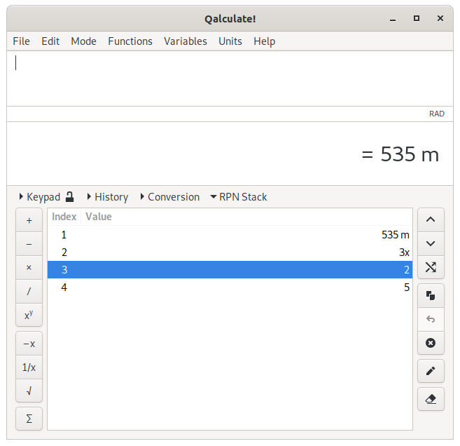
The RPN mode adds a third page to the main window, for display and manipulation of the values on the stack. This shows a list of values on the stack, with the last added value on the top.
On the right are buttons for manipulation of the stack. The buttons move the selected value up (Ctrl+Up) or down (Ctrl+Down), move it to the top (Ctrl+Right), copy it (Ctrl+Shift+C), edit it, or remove it (Ctrl+Delete), in order. If no stack row is selected, the up and down buttons rotates the stack, the swap button swaps the places of the first and second value and the copy and delete buttons acts on the top value of the stack. The button between copy and delete enters the top value from before the last numeric operation (Ctrl+Left). The last button removes all values from the stack (Ctrl+Shift+Delete).
On the left are buttons for applying mathematical operations to the stack. The top left buttons applies addition, subtraction, multiplication, division, and exponentiation to the top two values. If only one value is available addition, multiplication, and exponentiation uses this value twice, while the subtraction button negates the value and the division button calculates the reciprocal. The buttons below negates the top value, calculates the reciprocal, and calculates the square root of the top value. The last button calculates the sum of all values on the stack. Changes in the display of results only affects the first value on the stack.
Reverse Polish Notation can also be used directly in expression. This can be activated or deactivated separately from the RPN stack ( → → ). When using RPN syntax, a temporary stack, separate from the previously mentioned stack, is created from the contents of each mathematical expression entered. To calculate “(5 + 3)/2”, as in the example above, with RPN syntax you should enter the expression “5 3 + 2 /”. Instead of actually pressing enter on the keyboard, each separate value on the stack is separated by a blank space.
Two different algorithms for calculation of intervals or propagation of uncertainties are supported (selectable from +). This applies to numbers, defined using the interval() function or “±” notation, or with “read precision” enabled, and variables, including physical constants, with specified standard uncertainty. The uncertainty will be calculated separately for non-differentiable functions.
By default the variance formula is used. Intervals are with this method treated as values with measurement uncertainties (the value 5±0.01 has a standard deviation of 0.01). The final uncertainty, or error, is estimated using partial derivatives, as shown below. For expressions involving complex numbers, the imaginary uncertainty are calculated separately.
Alternatively interval arithmetic can be used. Intervals are treated as an absolute range of values and the result represents all possible values for every value within all ranges in the expression. For monotonic functions the endpoints in the result corresponds to the function values for the endpoints of the input (e.g. “interval(x, y)^3=interval(x^3, y^3)”).
Interval arithmetic is also used implicitly, regardless of selected interval calculation algorithm, for all approximate calculations to keep track of precision changes, and gracefully handle for example catastrophic cancellation (in subtraction two nearly equal numbers). The behavior can be (de)activated using + → .
Some non-invertible functions (including bessel and airy functions) do not properly support interval arithmetic and only the function values for the endpoints of the interval are calculated. Trigonometric functions returns correct intervals for real and imaginary numbers, but will in some cases for complex numbers with both a real and imaginary part return a too wide interval. Generally, the resulting interval will be guaranteed to include the true interval, but may for non-trivial expression (especially involving complex numbers) return an interval that is too wide.
The result is by default shown as an ordinary number with the number of significant digits determined by the size of the uncertainty (“2.11±0.03 = 2.1”), or the width of interval, unless the interval is too wide. If the interval() function has been used in the expression the result is by default displayed as an interval, and if “±” notation (or the uncertainty() function) has been used, it will also be used in the result. The default behavior can be changed from+. The midpoint alternative displays the value halfway between the lower and upper limit of the interval (“interval(2.075, 2.15) = 2.1125”). Note that, for the plus/minus notation, the same midpoint (note that when interval arithmetic is enabled this does not necessarily equal the result for the midpoint of intervals in the expression) is displayed in front of the plus/minus symbol. In plus/minus notation, the uncertainty is displayed with two significant digits, with the exception that all digits before the decimal separator are always shown.
Table of Contents
Variables are used to conveniently store a fixed value/result under a name. Variables can store everything that a result may contain, including numbers, units, variables, unsolved expressions and functions etc.
There are two different kinds of variables: known and unknown. Known variables represent a fixed value, usually a number, while unknown variables represent a range or type of values (e.g. a non-negative integer).
Some common constants that can only be approximately represented by a real number, such as pi and e, are special known variables. They are not fixed but are recalculated each time precision changes, thereby not compromising the arbitrary precision of Qalculate!.
The ans variable always contains the most recent result. For multiple results of an equation, this variable contains a vector of solutions (access the first solution using “ans(1)”).
The unknown variables x, y and z are predefined. They cannot be deleted, but changed. By default they use the default assumptions.
For a complete list of available variables see Appendix B, Variable List or the variable manager.
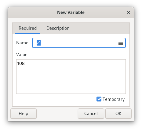
The easiest way to create a known variable is to store the current result. This can be done by clicking the button or selecting → . Type a name for the variable in the dialog that pops up. The name is used in expressions (e.g. “var_1 + 5” if the variable is named “var_1”). Temporary variables (placed in the “Temporary” category) disappear when Qalculate! is closed.
Known variables can also be created from scratch by selecting → → or by clicking in the variable manager. The value is entered in the text field below the name. Any mathematical expression is allowed as value (e.g. “π m” or “sin(2) + ln(3)”).
It is possible to specify multiple names, and various properties of these names, by clicking the icon on the right side of the name field.
The second page of the dialog provides fields for entry of descriptive name (shown as title in menus), category, and description.
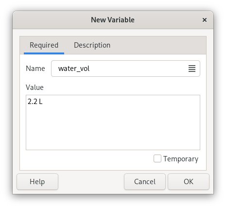
Alternatively values can be stored in variables using the save() function, or the associated “:=”/“=” operators (e.g. “save(v1, 5)” or “v1:=5”, “save(v1, ln(5)+2,,,1)” or “v1=ln(5)+2”).
The dialog for creation of unknown variables is accessed by selecting → → . Instead of a value, an assumed type and sign can then be selected.
Edit a variable by clicking in the variable manager, or using the context menu (right-click) of the corresponding menu item in the menu of the .
The special ( right-click) variable is updated using the classic ( right-click), (( middle-click), ( right-click), and ( middle-click) operations.
Vectors and matrices are most effectively used stored in a variable. Qalculate! provides separate tools for these variables. They use a different dialog, where each element can be edited separately as in a spreadsheet. As with other variables, click in the variable manager to edit a matrix/vector variable, but to create a new, select → → or → → .
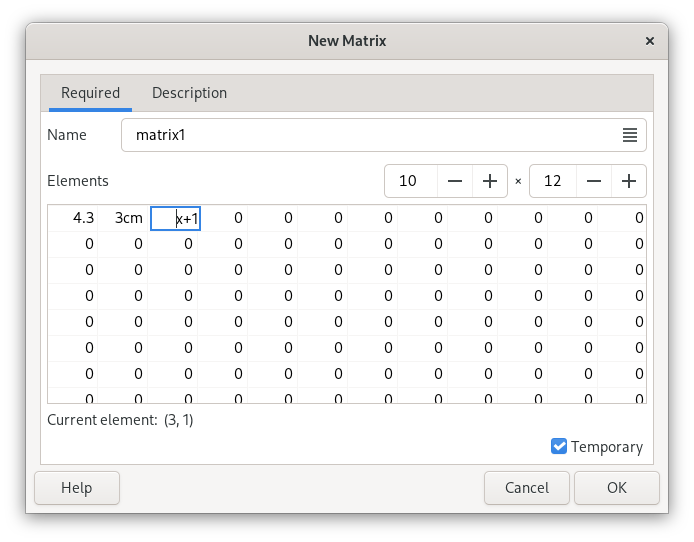
In this dialog, name, category and descriptive name are typed in as usual, but instead of a single value field, multiple values are entered using a table. The number of rows and columns are selected using the controls above the table. In a vector this only determines how many cells that are shown in the table and empty cells will be ignored. For matrices, each cell in the table is an element in the matrix.
Matrices and vectors can also be loaded from data files. These files must be plain text files with values organized in separated rows and columns. Select → and a dialog window pops up. First select the file to import and then specify whether it shall be imported as a matrix or vectors. A name, descriptive name and category can optionally be typed in. If the name field is empty, the file name will be used instead. After that, the row in the file where the data starts should be specified, as well as whether this first row contains column headings. Finally the delimiter, used to separate columns in the file, must be selected. Click and variables will be generated from the file. If vectors are to be generated and the file contains more than one column, the name will be used as a subcategory and each variable will add the column heading (or “Column 1”, “Column 2”, ...) to the name and the descriptive name.
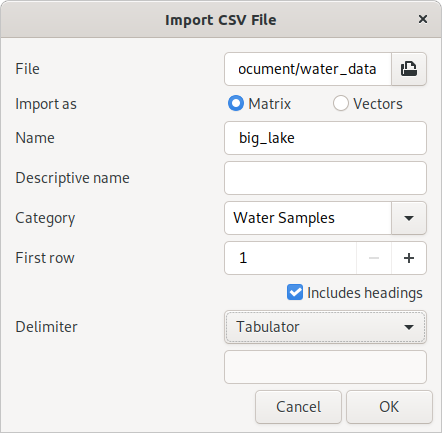
The load() function can be used to access a CSV file directly in an expression. The reversed action is also available with export(), or the dialog accessed with → or from the variable manager.
Table of Contents
Functions are essentially mathematical formulas. They are used to store expressions with variable values, arguments. To execute a function, the values for a number of arguments need to specified. These arguments are then inserted into the expression, making it possible to calculate.
Functions are normally entered in an expression by writing the name followed by arguments, separated by commas (or semicolons in languages with comma as decimal point), in parenthesis, thus following the syntax name(arg1, arg2, ...). Qalculate! will give a helpful error message if the arguments are not correct.
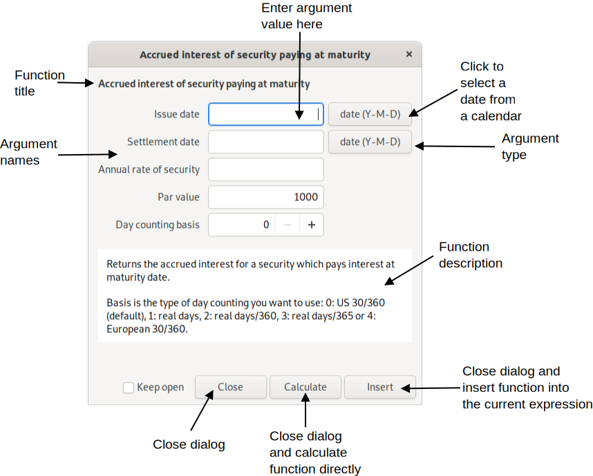
The insert function dialog presents an easy way to insert a function and its arguments.
Although it can lower the readability of an expression, it is perfectly legal to skip the parenthesis and put the arguments after a space, and end with a space or operator. This is most useful in short expressions with single argument functions (e.g. “sqrt 5”).
Argument types include:
Free — anything
Number — a numeric value
Integer — a whole number
Symbol — a defined or undefined unknown variable
Text — a free text string
Date — a date in local or standard format (Year-Month-Day, recommended)
Vector
Matrix
Boolean — 0 for false, 1 for true
Object — the name of a variable, function or unit
Variable — the name of a variable
Function — the name of a function
Unit — the name of a unit
File — the path to a file
Angle — an angle used in trigonometric functions, meaning a number and an angle unit. If no angle unit is included the default is used.
The argument can be restricted by further conditions. For example that a number must be positive.
Most arguments (primarily number arguments) can be replaced by a vector. The function will then be calculated for each vector element and a new vector will be returned. If more than one argument are supplied to a function that takes exactly one argument, each argument will be treated as elements of a vector.
Here the main function categories and some of their members are described, to give an overview of available functions. For information about separate functions and a complete list of all available functions see Appendix A, Function List or the function manager.
- Algebra
Contains sum() and product(), which corresponds to the sum and product signs. solve() solves equations (e.g. “solve(x × 2 = 8)” returns “4” meaning that x equals 4). Use solve2() and multisolve() to solve multiple equations with multiple variables.
- Calculus
Includes diff(), which calculates the derivative of an expression with optional arguments “with respect to” (default x) and “order” (default 1), and a limited integration function.
- Combinatorics
Contains functions such as perm() for permutations, comb() for combinations, and factorial().
- Complex Numbers
Contains functions useful for calculations with complex numbers, including arg() for principal argument and conj() for conjugate.
- Data Sets
A data set consists of a set of properties and objects, which can be accessed by a function which takes two arguments — object and property. The function returns the object's value for the selected property. For example, the data in the “Elements” data set is accessed with the atom() function, with the element (referenced using atomic symbol, number or name) and property (e.g. weight) as arguments. The special property “info” displays all properties of the object in a dialog window.
- Date & Time
Includes days() and yearfrac() which returns the number of days and fractional years, respectively, between two dates.
- Exponents & Logarithms
Standard logarithmic and exponential functions. ln() calculates the natural logarithm of a number, while log() allows a choice of base as the second argument. The cbrt() and root() functions only calculates real roots. For roots of odd degree the root functions give a different answer than the exponential operator, “^”, for negative values (“cbrt(-8) = -(8)^(1/3) = -2”, but “(-8)^(1/3) = 1 + 1.73i”).
- Economics
This essentially includes most of the financial functions that are usually found in spreadsheet applications.
- Elements
This category includes functions to retrieve data such as atomic weight. The atom() function opens a window with available data of an element. These functions accept the number, symbol or name of the element as argument. The data are loaded on demand.
- Geometry
Category with formulas mostly for calculation of circumference, area and volume of geometric shapes.
- Logical
Some procedural functions mainly for use in other functions. These include if(), which tests a conditional expression and returns a value depending on if the expression evaluates true or false, and for(), which processes a value while a condition is true.
- Matrices & Vectors
These are functions that generate, access and process matrices and vectors. The vector() function generates a vector from a variable number of arguments for elements, while matrix() first needs the number of rows and columns and then the elements from left to right. Matrices can also be imported directly from a CSV file with load().
Separate elements at a specified row and column are accessed with element(). Other functions include det() for calculation of the determinant of a matrix and inverse() which returns the inverse of the given matrix, as well as functions such as sort() and rank().
- Miscellaneous
A category for functions that do not fit elsewhere.
- Number Theory
Contains subcategories arithmetic, number bases, and rounding, in addition to functions such as abs(), which returns the absolute value of a number (“|” can also be used; e.g. “|-5| = abs(-5) = 5”, and gcd(), the greatest common divisor. round() is the standard rounding function. The functions for number bases translates a text string, representing an expression with numbers in a different base, to a decimal number. Includes bin() for binary numbers, hex() for hexadecimal numbers, oct() for octal numbers and base() for numbers in a any other base.
- Special Functions
Includes beta(), gamma() and similar functions, as well as Riemann zeta (zeta()) and Kronecker delta (kronecker()).
- Statistics
Contains a lot of functions for descriptive statistics and some statistical tests. Data sets are stored as vectors. Generally, functions with a vector/data set as last argument can take elements/samples as a variable number of arguments directly instead of in a vector (e.g. “mean(1, 2, 3)” equals “mean(vector(1, 2, 3))”). Also contains the rand() function, which returns a pseudo random number between 0 and 1 (with no argument, or zero), or a random integer between one and the specified number.
- Trigonometry
Trigonometric functions, including sin(), cos(), tan(), sec(), csc(), cot(), and hyperbolic and inverse versions of those. These functions take as argument an angle. If the default angle unit ( → ) is set to none, the argument must have an angle unit appended (degrees, radians or gradians), otherwise the default unit will be appended automatically (and removed from result of inverse functions).
- Utilities
Various utility functions. Most are only useful in definition of other functions. The save() function can however be a quick way of storing a value in a variable, and csum() can be a powerful tool for data processing. This category also contains some functions, such as char() and ascii(), that might be useful for programmers. replace() provides an easy way of replacing unknown variables by known expressions in a value (e.g. “replace(5x^2 + x, x, 3)” equals “5 × 3^2 + 3”).
Functions are a bit more complex than variables, but can nevertheless be relatively easily created. Select → → , or click the on the keypad or in the function manager and a function edit dialog pops up.
The function edit dialog is divided in three pages, where the first page contains the only required properties — name and an expression. x, y and z with or without (default) a backslash are used as argument placeholders in the expression.
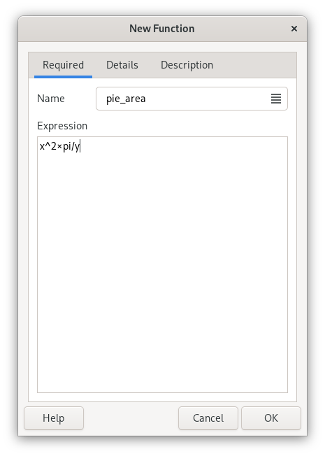
First enter a name, used to reference the function in an expression. Then enter an expression below.
The expression of a function is basically a normal expression with placeholders for arguments. The expression “x^4” creates a function which calculates the fourth power of a single argument. If you name it for example “sqsq”, “sqsq(2)” will calculate “2^4”.
The argument placeholders consist of a backslash and a letter — x, y, z for the 1st, 2nd and 3rd arguments and a to u for argument 4 to 24. The backslash can however be omitted, but avoids any possible conflict with existing variables, units and functions used in the expression. The argument symbols are replaced by entered arguments when a function is calculated. They also decide the number of arguments that a function requires. For example the function for triangle area (“base × height / 2”) has the name triangle and the expression “(\x × \y)/2”, which gives that “triangle(2, 3)” equals “(2 × 3) / 2” and returns “3” as result. An argument can be used more than one time and all arguments must not necessarily be in order in the expression.
Additionally, optional arguments can be put in the expression with upper-case (X, Y, Z, ...) instead of lower-case letters (x, y, z, ...). The default value should be put in curly brackets after the letter (e.g. “\X{2}”). The default value may be omitted and is then zero. All additional arguments after an optional argument must also be optional.
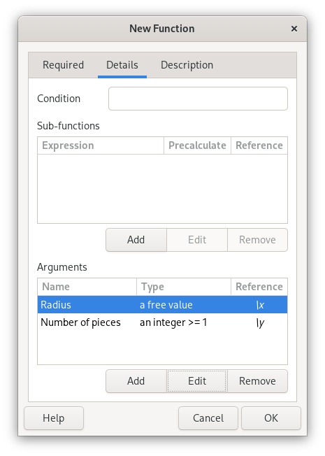
A required condition, sub-functions, and argument definitions can optionally be specified in the second page (“Details”).
The condition specifies an expression which must evaluate true before the function is calculated. This follows the same conventions as function expressions. For example, if the value of the second argument must be higher than the first, “\y > \x” may be entered as a condition.
Sub-functions can be useful for complex functions, they use the same syntax as the main expression, and are references using a backslash followed by a number (e.g. “\1” for the first sub-function). The sub-function can be inserted in the main expression as a precalculated value or intact (meaning that the subfunction might be recalculated for each occurrence in the main expression).
Name, type, and required conditions can be specified for each argument.
The third page allows entering of category, descriptive name (shown as title in menus) and description. The function can also be hidden from menus with the corresponding check box, which can be useful for functions only used in other functions.
Global, system-wide functions can not actually be changed by the user, but if one of these functions is edited, they are deactivated and seemingly replaced by a new function. Some functions are however hard-coded and cannot be changed by the user. Once the user function is removed or deactivated the original function is automatically reactivated.
Table of Contents
Units give numbers meaning in the real world. They specify what is measured by the numbers and the scale used. Qalculate! fully incorporates units in calculations and includes all standard SI units as well as many non-standard local units. For a complete list of available units see Appendix C, Unit List or the unit manager.
Among units, Qalculate! has support for currencies with up-to-date exchange rates. Currencies are normally referenced with the standard three letter code due to name clashes, but a number of currency unit can also be accessed through their regular name and symbol. U.S. dollars can, for example, be referenced both as USD and dollar/dollars or the $ symbol, unless the same name and/or symbol are used by the local currency.
The exchange rates can be updated manually using → , or automatically at specific intervals (by default once every week, but this can be changed in the preferences dialog), when needed (when currencies are converted).
Expressions can be converted to a specific unit directly in the expression entry with the “to” operator (right arrows, including “->” are also supported), which converts the left-hand expression (or the previous result) to a specified unit (e.g. “5 feet + 2 inches to cm” converts the result of “5 feet + 2 inches” to centimeters). Unit expressions may contain units, prefixes, exponents, multiplication and division. By default, no prefix will be added to units typed without prefix, but this behavior can be modified by putting a question mark in front of the unit expression (“6 561 ft to m ≈ 2000 m” but “6 561 ft to ?m ≈ 2 km”). Type “to optimal” to get optimal unit, “to base” for base units, or “to mixed” to force the use of mixed units (see below). Note that the conversion is always applied to the whole left-hand expression, ignoring any unmatched parentheses. The “to” operator can also be used for other types of result transformations (see the section called “The “to” (and “where”) operators”).
Alternatively the unit conversion view can be used. It is opened using Conversion, Ctrl+O, → or Ctrl+T (the last two options moves the focus to the unit expression entry). Enter a unit expression in the text entry and press Enter (or click ), or select a unit from the list. An appropriate unit category will automatically be selected from units in the current result. If is checked subsequent results will automatically be converted (if the conversion view is open), and if is checked the optimal prefix will be set for unit expressions without any prefix. A unit can be inserted directly into the expression entry from the list using middle click or the context menu.
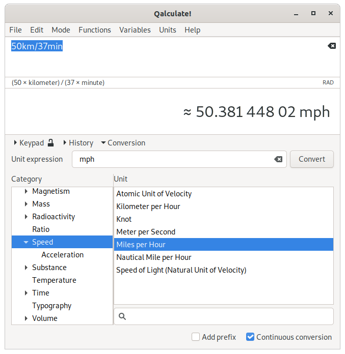
The result context menu and the menu associated with the keypad button also provides a list of units for conversion.
The final way to convert the result to another unit is to use → menu or to press in the unit manager, which also provides quick conversion of a value between two selected units. → can be used to select a prefix.
It is also possible to let Qalculate! automagically convert the result to appropriate units with → or → (or the corresponding options in the result context menu). If instead the corresponding choice is selected from + (or the result context menu), each result will automatically be converted until the choice is deactivated (+ → ).
By default (controlled by → → ) certain units, such as time units and many imperial/U.S. customary units, are automatically converted to mixed units (e.g. “60.2 minutes = 1 hour to 12 seconds”). When explicitly converting to a specific unit the integer value of the selected unit is preserved (“1.51 h to min = 90 min + 36 s”) and mixed units is not used if otherwise the unit would not be present in the result (“6 in to ft = 0.5 ft”). This behavior can be modified by prepending the unit with a plus or minus sign (e.g. “174 cm to +in ≈ 5 ft + 8,5 in”, “1.51 h to -min = 90.6 min”).
There are three different unit classes in Qalculate! — base units, named derived units, and (unnamed) derived units. Base units are standard units that form the basis for all other units. Meters and seconds are typical base units. Derived units are defined in relation to other units. Named derived units are defined in relation to a single other unit, with an optional exponent (e.g. hour is defined as a named derived unit that equals 60 minutes which in turn is defined in relation to seconds). Unnamed derived units are defined by a unit expression with one or multiple units (e.g. “J/s”). They are primarily useful as basis for named derived units (e.g. W = J/s), and for simplified conversion and entry of the specified unit expression.
Select → → , or click in the unit manager, and the unit edit dialog pops up.
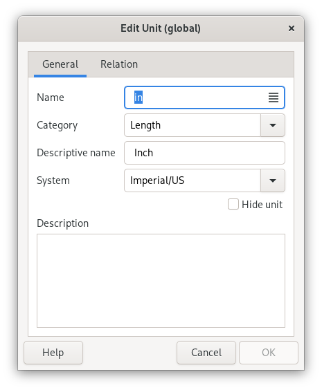
Base units and named derived units normally have three different name forms defined for use in expressions — abbreviation (e.g. “m”), singular (“meter”) and plural (“meters”). Unnamed derived units only have an internal name, which is used to reference the unit in definitions of other units, but which should not be used in mathematical expressions.
In addition category and descriptive name can be specified to keep the units well organized. A unit can be hidden from unit menus with the corresponding check box (this is primarily useful for some unnamed derived units which are only defined as basis for named derived units).
Depending on the unit class, different elements in the relation page of the dialog will be enabled.
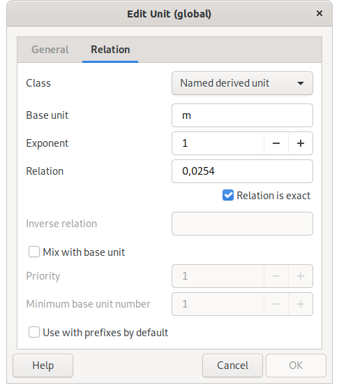
For named derived units, base unit, exponent and relation must all be specified (although the exponent and relation may both be left as “1”). The base unit can be of any unit class and it is recommended that named derived units are defined in relation to the closest unit (e.g. 1 ft = 3 hands, 1 hand = 4 in, and 1 in = 0.0254 m). The relation is usually just a number that tells how large quantity of the base unit is needed to get the derived unit (derived unit = relation × base unitexponent).
It is possible to create units with non-linear relation to the base unit. Replace the factor with “\x” and the exponent with “\y” (e.g. “\x + 273.15” for degrees Celsius with Kelvin as base unit). For non-linear relations the reverse relation (for conversion back from the base unit) should also be specified (“\x - 273.15” for degrees Celsius).
Base unit mixing can be enabled (by default) for named derived units. This is used for units such as feet and minutes, which are often combined with other units instead of using decimals (e.g. “5.25 ft = 5 ft + 3 in”, “250 s = 4 min + 10 s”). This behavior can be fine-tuned using the priority and minimum base unit number properties.
For unnamed derived units a unit expression, with one or multiple units, must be specified in the base units field. This expressions may only contain units, prefixes, exponents, multiplication and division (e.g. “km/h”).
Plotting in Qalculate! is done through an external program, Gnuplot. Thus Gnuplot needs to be installed separately, and found in the executable search path, for plotting to work.
To plot functions or data sets, select → , which brings up the plot dialog. The plot dialog consists of three tabs/pages — the first for the data, the second for the function range and sampling rate, and the last for control of function sampling and appearance.
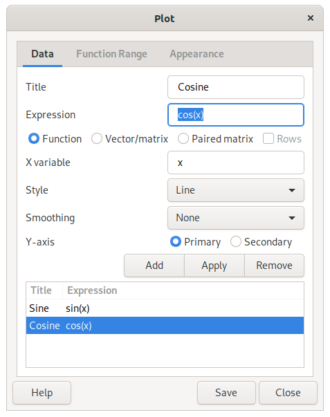
Plot functions are normal expressions that represent f(x) in y=f(x) (e.g. “sin(x)”). The x can be specified as a different unknown variable (x, y, z) or a quoted text string (actually any mathematical expression which will then be matched in the plot expression and replaced by the values on the x axis) in the variable entry below the function/data list.
To plot a data set, enter an expression that results in a matrix or vector. Select Vector/Matrix below and vectors will appear as one series and matrices will appear with each column or row (if selected) as a series, If the paired matrix option instead is selected, the first column/row of the matrix will constitute the y-values and the second the x-values.
Type in an expression, press Enter and a new window will open with the plot. The title of the series, the diagram style and smoothing of the line can also be set. The series modified must be selected in the list and to apply changes click . More series that will appear in the same plot window can be added. If the scale of the y values differ, series can be put on a secondary y-axis.
Caution
Even though Qalculate! does all the calculations before handing over the data to Gnuplot, the resulting data must only consist of pure numbers, as Gnuplot knows nothing about the functions, variables, units, etc. of Qalculate!.
For functions, the function range — min and max x value, and the number of values or the size of the step between each y value calculated — can be specified in the function range page.
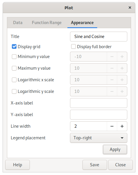
A title can be set to appear at the top of the plot, as well as labels for the x and y axis. The appearance can also be controlled by selecting or disabling legend placement, displaying/hiding the grid and borders on the top and the right side of the diagram and choosing color or monochrome graphics. The x and y scales can be made logarithmic by clicking the box on the right and filling in a desired logarithmic base.
To update the plot window, click at the bottom of the dialog.
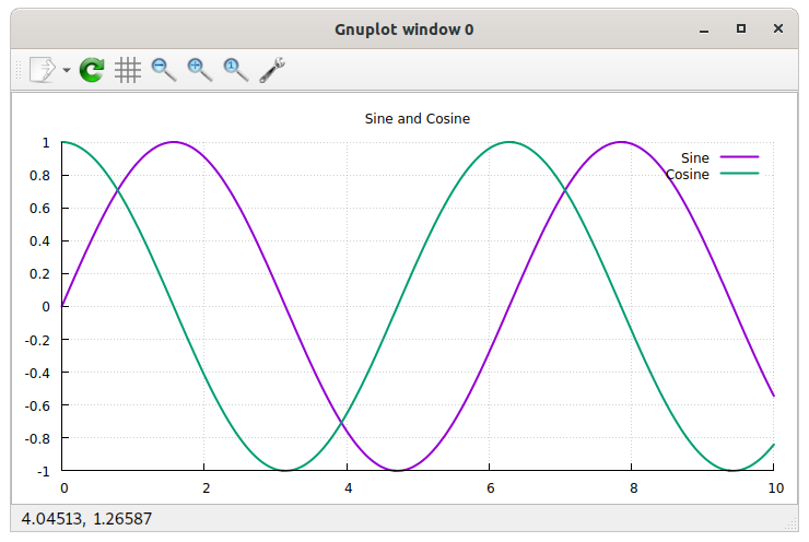
The plot can be saved as an image file. Click and select a file name and folder. The extension of the file name will decide the file type (.png for PNG image, .svg for SVG, .ps for postscript, .eps for encapsulated postscript, .tex for LaTeX, and .fig for XFig). Default is to save as a PNG image.
Table of Contents
- Find Linear Function
linearfunction(x1, y1, x2, y2)
Finds the linear function for the straight line between two distinct points.
Arguments.
x1: a free value
y1: a free value
x2: a free value
y2: a free value
- Product of a sequence
product(Factor expression, Lower limit (i), Upper limit (n)[, Index variable])
Π
Corresponds to the product symbol. Multiplies factors for each x ranging from the lower to the upper limit.
Example: product(x2, 1, 5) = 12 × 22 × 32 × 42 × 52 = 14400
Arguments.
Factor expression: a free value
Lower limit (i): an integer
Upper limit (n): an integer
Index variable: an unknown variable/symbol (optional, default: undefined)
Requirement. "Upper limit (n)" ≥ "Lower limit (i)"
- Solve differential equation
dsolve(Equation[, Initial condition: function value (y)][, Initial condition: argument value (x)])
Solves a differential equation and returns the value of y(x). The derivative in the equation should be in the format diff(y, x). Only first-order differential equations are currently supported.
Example: dsolve(2 × diff(y, x) − y = 4x, 5, 2) = 21e^(x/2) / e − 4x − 8
Arguments.
Equation: a free value
Initial condition: function value (y): a free value (optional, default: undefined)
Initial condition: argument value (x): a free value (optional, default: 0)
- Solve equation
solve(Equation[, With respect to])
Arguments.
Equation: a free value
With respect to: an unknown variable/symbol (optional, default: undefined)
- Solve for multiple variables
multisolve(Equation vector, Variable vector)
Arguments.
Equation vector: a vector
Variable vector: a vector with an unknown variable/symbol, ...
Requirement. dimension("Equation vector") = dimension("Variable vector")
- Solve for two variables
solve2(Equation 1, Equation 2[, Variable 1][, Variable 2])
Solves two equations with two unknown variables. Returns the value of the first variable.
Arguments.
Equation 1: a free value
Equation 2: a free value
Variable 1: an unknown variable/symbol (optional, default: x)
Variable 2: an unknown variable/symbol (optional, default: y)
- Solve using Newton's Method
newtonsolve(Equation, Initial estimate[, Variable][, Precision][, Max iterations])
Arguments.
Equation: a free value
Initial estimate: a number
Variable: an unknown variable/symbol (optional, default: undefined)
Precision: an integer ≥ -2147483648 and ≤ 2147483647 (optional, default: -10)
Max iterations: an integer ≥ 0 and ≤ 4294967295 (optional, default: 1000)
- Solve using Secant Method
secantsolve(Equation, Initial estimate 1, Initial estimate 2[, Variable][, Precision][, Max iterations])
Arguments.
Equation: a free value
Initial estimate 1: a number
Initial estimate 2: a number
Variable: an unknown variable/symbol (optional, default: undefined)
Precision: an integer ≥ -2147483648 and ≤ 2147483647 (optional, default: -10)
Max iterations: an integer ≥ 0 and ≤ 4294967295 (optional, default: 1000)
- Summation
sum(Term expression, Lower limit (i), Upper limit (n)[, Index variable])
Σ
∑
Corresponds to the summation symbol. Adds terms for each x ranging from the lower to the upper limit.
Example: sum(x2, 1, 5) = 12 + 22 + 32 + 42 + 52 = 55
Arguments.
Term expression: a free value
Lower limit (i): an integer
Upper limit (n): an integer
Index variable: an unknown variable/symbol (optional, default: undefined)
Requirement. "Upper limit (n)" ≥ "Lower limit (i)"
- Differentiate
diff(Function[, With respect to][, Order][, Variable value])
derivative
Arguments.
Function: a free value
With respect to: an unknown variable/symbol (optional, default: undefined)
Order: an integer ≥ 1 and ≤ 2147483647 (optional, default: 1)
Variable value: a free value (optional, default: undefined)
- Extreme Values
extremum(Function[, With respect to])
Arguments.
Function: a free value
With respect to: an unknown variable/symbol (optional, default: x)
- Integrate
integrate(Function[, Lower limit][, Upper limit][, Variable of integration][, Force numerical integration])
integral
∫
Arguments.
Function: a free value
Lower limit: a free value (optional, default: undefined)
Upper limit: a free value (optional, default: undefined)
Variable of integration: an unknown variable/symbol (optional, default: undefined)
Force numerical integration: a boolean (0 or 1) (optional, default: 0)
- Limit
limit(Function, Value to approach[, Variable][, Direction])
Returns the two-sided limit of the function if direction is zero, limit from left (below) if direction is -1, or limit from right (above) if direction is +1.
Arguments.
Function: a free value
Value to approach: a real number
Variable: an unknown variable/symbol (optional, default: x)
Direction: an integer ≥ -1 and ≤ 1 (optional, default: 0)
- Limit with Multiple Variables
multilimit(Function, Variable vector, Value vector[, Direction vector])
Returns limit of a function for multiple variables. The limit is calculated recursively, for one variable in each iteration, with the result of each iteration used as function in the next.
Example: multilimit(x2/(x+y)×y, [x y], [−2 1]) = −4
Arguments.
Function: a free value
Variable vector: a vector
Value vector: a vector
Direction vector: a vector (optional, default: 0)
Requirement. dimension("Variable vector")=dimension("Value vector")
- Romberg Integration
romberg(Function, Lower limit, Upper limit[, Min iterations][, Max iterations][, Variable of integration])
Arguments.
Function: a free value
Lower limit: a real number
Upper limit: a real number
Min iterations: an integer ≥ 2 and ≤ 9223372036854775807 (optional, default: 6)
Max iterations: an integer ≥ -9223372036854775808 and ≤ 9223372036854775807 (optional, default: 20)
Variable of integration: an unknown variable/symbol (optional, default: undefined)
Requirement. "Upper limit" > "Lower limit"
- Cosine Integral
Ci(argument)
cosint
The integral of cos(x)/x.
Arguments.
1: a number
- Exponential Integral
Ei(argument)
expint
The integral of e^x/x.
Arguments.
1: a number
- Fresnel Integral C
fresnelc(argument)
The integral of cos(pi*x^2/2).
Arguments.
1: a number ≥ -6 and ≤ 6
- Fresnel Integral S
fresnels(argument)
The integral of sin(pi*x^2/2).
Arguments.
1: a number ≥ -6 and ≤ 6
- Hyperbolic Cosine Integral
Chi(argument)
coshint
The integral of cosh(x)/x.
Arguments.
1: a number
- Hyperbolic Sine Integral
Shi(argument)
sinhint
The integral of sinh(x)/x.
Arguments.
1: a number
- Inverse Regularized Incomplete Beta Function
betaincinv(argument 1, argument 2, argument 3)
Arguments.
1: a number ≥ 0 and ≤ 1
2: a number
3: a number
- Logarithmic Integral
li(argument)
logint
The integral of 1/ln(x).
Arguments.
1: a number
- Lower Incomplete Gamma Function
gammainc(argument 1, argument 2)
Arguments.
1: a free value
2: a free value
- Regularized Incomplete Beta Function
betainc(argument 1, argument 2, argument 3)
Arguments.
1: a real number
2: a real number
3: a real number
- Sine Integral
Si(argument)
sinint
The integral of sin(x)/x.
Arguments.
1: a number
- Upper Incomplete Gamma Function
igamma(argument 1, argument 2)
Arguments.
1: a number ≥ -100000 and ≤ 1000000
2: a number ≤ 1000
- Binomial Coefficient
binomial(n, k)
Arguments.
n: a real number
k: a real number
- Combinations
comb(Objects, Size)
Returns the number of possible arrangements of an unordered list with a number of objects to choose from and a list size. If there are three objects (1, 2 and 3) that are put in a list with place for two, the alternatives are [1, 2], [1, 3], and [2, 3], and thus the number of combinations is 3.
Arguments.
Objects: a number
Size: a number
- Derangements
derangements(Number of elements)
Returns the number of possible rearrangements of an ordered list, of a certain size, where none of the objects are in their original positions. If the original list is [1, 2, 3], the possible derangements are [2, 3, 1] and [3, 1, 2], and thus the number of derangements is 2.
Arguments.
Number of elements: an integer ≥ 1
- Double Factorial
factorial2(Value)
Calculates the double factorial of an integer. Multiplies the argument with every second lesser positive integer (n(n-2)(n-4)...). Can also be entered as a number followed by two exclamation marks.
Example: factorial2(5) = 5!! = 5 × 3 × 1 = 15
Arguments.
Value: an integer ≥ -1 and ≤ 9223372036854775807
- Factorial
factorial(Value)
Calculates the factorial of an integer. Multiplies the argument with every lesser positive integer (n(n-1)(n-2)...2*1). Can also be entered as a number followed by one exclamation mark.
Example: factorial(5) = 5! = 5 × 4 × 3 × 2 × 1 = 120
Arguments.
Value: an integer ≥ 0 and ≤ 9223372036854775807
- Hyperfactorial
hyperfactorial(Value)
Calculates the hyperfactorial of an integer. Multiplies the argument raised by itself with every lesser positive integer raised by themselves (1^1 * 2^2 ... n^n).
Example: hyperfactorial(3) = (33) × (22) × (11) = 108
Arguments.
Value: an integer ≥ 1
- Multifactorial
multifactorial(Value, Factorial)
Calculates the multifactorial of an integer. Multiplies the argument with every x lesser positive integer (n(n-x)(n-2x)...). Can also be entered as a number followed by three or more exclamation marks.
Example: multifactorial(18, 4) = 18!!!! = 18 × 14 × 10 × 6 × 2 = 30 240
Arguments.
Value: an integer ≥ 0 and ≤ 9223372036854775807
Factorial: an integer ≥ 1 and ≤ 9223372036854775807
- Permutations (Variations)
perm(Objects, Size)
variations
Returns the number of possible arrangements of an ordered list with a number of objects to choose from and a list size. If there are three objects (1, 2 and 3) that are put in a list with two positions, the alternatives are [1, 2], [2, 1], [1, 3], [3, 1], [2, 3] and [3, 2], and thus the number of permutations is 6.
Arguments.
Objects: a number
Size: a number
- Superfactorial
superfactorial(Value)
Calculates the superfactorial of an integer. Multiplies the factorial of the argument with the factorial of every lesser positive integer (1! * 2! ... n!).
Example: superfactorial(5) = 5! × 4! × 3! × 2! × 1! = 34 560
Arguments.
Value: an integer ≥ 0
- Complex Conjugate
conj(Complex number)
Arguments.
Complex number: a number
- Imaginary Part
im(Complex number)
ℑ
Arguments.
Complex number: a number
- Principal Argument
arg(Complex number)
Arguments.
Complex number: a number
- Real Part
re(Complex number)
ℜ
Arguments.
Complex number: a number
- Elements
atom(Element[, Property])
Retrieves data from the Elements data set for a given object and property. If "info" is typed as property, all properties of the object will be listed.
This data uses material from the Wikipedia, under the Creative Commons Attribution-ShareAlike License
Arguments.
Element: an object from "Elements" (use symbol, number, or name)
Property: name of a data property (symbol, number, name, mass, boiling, melting, or density) (optional, default: info)
Properties.
Symbol: symbol (key)
Number: number (key)
Name: name (key)
Atomic Mass: mass, weight
The property uses standard atomic weight, when determined, or the mass number.
Boiling Point: boiling
Melting Point: melting
Density: density
Density at STP (gases) or near room temperature
- Planets
planet(Planet[, Property])
Retrieves data from the Planets data set for a given object and property. If "info" is typed as property, all properties of the object will be listed.
This data uses material from the Wikipedia articles
"Earth" (http://www.wikipedia.org/wiki/Earth),
"Jupiter" (http://www.wikipedia.org/wiki/Jupiter),
"Mars" (http://www.wikipedia.org/wiki/Mars),
"Mercury (planet)" (http://www.wikipedia.org/wiki/Mercury_(planet)),
"Neptune" (http://www.wikipedia.org/wiki/Neptune),
"Pluto" (http://www.wikipedia.org/wiki/Pluto),
"Saturn" (http://www.wikipedia.org/wiki/Saturn),
"Uranus" (http://www.wikipedia.org/wiki/Uranus), and
"Venus" (http://en.wikipedia.org/wiki/Venus), under Creative Commons Attribution-ShareAlike License
Arguments.
Planet: an object from "Planets" (use name)
Property: name of a data property (name, year, speed, eccentricity, inclination, satellites, mass, density, area, gravity, temperature, or radius) (optional, default: info)
Properties.
Name: name (key)
Orbital Period (Year): year
Average Orbital Speed: speed
Eccentricity: eccentricity
Inclination (to ecliptic): inclination
Number of Satellites: satellites
Mass: mass
Mean Density: density
Surface Area: area
Equatorial Gravity: gravity
Mean Surface Temperature: temperature
Mean Radius: radius
- Add Days
addDays(Date, Days)
Arguments.
Date: a date (Y-M-D)
Days: a number
- Add Months
addMonths(Date, Months)
Arguments.
Date: a date (Y-M-D)
Months: a number
- Add Time
addTime(Date, Time)
Adds a time value to a date. The value can be positive or negative, but must use a unit based on seconds (such as day and year).
Example: addTime(today, 10 d) = today + 10 d; addTime(2025−10−05T07:48, 10 min) = "2025−10−05T07:48" + 10 min = "2025−10−05T07:58"
Arguments.
Date: a date (Y-M-D)
Time: a free value that fulfills the condition "isNumber(Time/s)"
- Add Years
addYears(Date, Years)
Arguments.
Date: a date (Y-M-D)
Years: a number
- Construct Date
date(Year[, Month][, Day][, Calendar])
Returns a date. Available calendars are gregorian (1), hebrew (2), islamic (3), persian (4), indian (5), chinese (6), julian (7), milankovic (8), coptic (9), ethiopian (10), egyptian (11). The Chinese year uses an epoch of 2697 BCE and chinese leap months are indicated by adding 12 to the month number (e.g. leap month 4 = 16).
Arguments.
Year: an integer ≥ -9223372036854775808 and ≤ 9223372036854775807
Month: an integer ≥ 1 and ≤ 24 (optional, default: 1)
Day: an integer ≥ 1 and ≤ 31 (optional, default: 1)
Calendar: a text string (optional, default: gregorian)
- Construct Date and Time
datetime(Year[, Month][, Day][, Hour][, Minute][, Second])
Arguments.
Year: an integer ≥ -9223372036854775808 and ≤ 9223372036854775807
Month: an integer ≥ 1 and ≤ 12 (optional, default: 1)
Day: an integer ≥ 1 and ≤ 31 (optional, default: 1)
Hour: an integer ≥ 0 and ≤ 23 (optional, default: 0)
Minute: an integer ≥ 0 and ≤ 59 (optional, default: 0)
Second: a number ≥ 0 and < 61 (optional, default: 0)
- Current Time
time()
- Date to Unix Timestamp
timestamp([Date])
Arguments.
Date: a date (Y-M-D) (optional, default: now)
- Day of Month
day([Date])
Arguments.
Date: a date (Y-M-D) (optional, default: today)
- Day of Week
weekday([Date][, Week begins on Sunday])
Arguments.
Date: a date (Y-M-D) (optional, default: today)
Week begins on Sunday: a boolean (0 or 1) (optional, default: 0)
- Day of Year
yearday([Date])
Arguments.
Date: a date (Y-M-D) (optional, default: today)
- Days between two dates
days(First date, Second date[, Day counting basis][, Financial function mode])
Returns the number of days between two dates.
Basis is the type of day counting you want to use: 0: US 30/360, 1: real days (default), 2: real days/360, 3: real days/365 or 4: European 30/360.
Arguments.
First date: a date (Y-M-D)
Second date: a date (Y-M-D)
Day counting basis: an integer ≥ 0 and ≤ 4 (optional, default: 1)
Financial function mode: a boolean (0 or 1) (optional, default: 0)
- Days in Month
daysInMonth([Date])
Arguments.
Date: a date (Y-M-D) (optional, default: today)
- Find Lunar Phase
nextlunarphase(Lunar phase[, Start date])
Returns the date when the specified lunar phase occurs. The function searches forward beginning at the specified date. The lunar phase is specified as a number between 0 and 1, where 0 represents new moon, 0.5 full moon, and 0.25 and 0.75 quarter moons. Angle values are also allowed (e.g. π rad = 180° which corresponds to a value of 0.5). Values above 1, without unit, are interpreted as degrees.
Arguments.
Lunar phase: a number ≥ 0 and < 1
Start date: a date (Y-M-D) (optional, default: now)
- Lunar Phase
lunarphase([Date])
Returns the lunar phase, as a number between 0 and 1, for the specified date. This value corresponds to an angle between 0 and 360 degrees. 0 represents new moon, 0.5 full moon, and 0.25 and 0.75 quarter moons.
Arguments.
Date: a date (Y-M-D) (optional, default: now)
- Month
month([Date])
Arguments.
Date: a date (Y-M-D) (optional, default: today)
- Time Value
timevalue([Date])
Returns the time part, in fractional hours, of a date and time value.
Arguments.
Date: a date (Y-M-D) (optional, default: now)
- Unix Timestamp to Date
stamptodate(Timestamp)
unix2date
Returns the local date and time represented by the specified Unix timestamp (seconds, excluding leap seconds, since 1970-01-01). Supports time units.
Arguments.
Timestamp: a free value
- Week of Year
week([Date][, Week begins on Sunday])
Arguments.
Date: a date (Y-M-D) (optional, default: today)
Week begins on Sunday: a boolean (0 or 1) (optional, default: 0)
- Year
year([Date])
Arguments.
Date: a date (Y-M-D) (optional, default: today)
- Years between two dates
yearfrac(First date, Second date[, Day counting basis][, Financial function mode])
Returns the number of years (fractional) between two dates.
Basis is the type of day counting you want to use: 0: US 30/360, 1: real days (default), 2: real days/360, 3: real days/365 or 4: European 30/360.
Arguments.
First date: a date (Y-M-D)
Second date: a date (Y-M-D)
Day counting basis: an integer ≥ 0 and ≤ 4 (optional, default: 1)
Financial function mode: a boolean (0 or 1) (optional, default: 0)
- Accrued interest of security paying at maturity
accrintm(Issue date, Settlement date, Annual rate of security[, Par value][, Day counting basis])
Returns the accrued interest for a security which pays interest at maturity date.
Basis is the type of day counting you want to use: 0: US 30/360 (default), 1: real days, 2: real days/360, 3: real days/365 or 4: European 30/360.
Arguments.
Issue date: a date (Y-M-D)
Settlement date: a date (Y-M-D)
Annual rate of security: a free value
Par value: a free value (optional, default: 1000)
Day counting basis: an integer ≥ 0 and ≤ 4 (optional, default: 0)
- Accrued interest of security with periodic interest payments
accrint(Issue date, First interest, Settlement date, Annual rate of security, Par value, Frequency[, Day counting basis])
Returns accrued interest for a security which pays periodic interest.
Allowed frequencies are 1 - annual, 2 - semi-annual or 4 - quarterly. Basis is the type of day counting you want to use: 0: US 30/360 (default), 1: real days, 2: real days/360, 3: real days/365 or 4: European 30/360.
Arguments.
Issue date: a date (Y-M-D)
First interest: a date (Y-M-D)
Settlement date: a date (Y-M-D)
Annual rate of security: a free value
Par value: a free value
Frequency: an integer ≥ 1 and ≤ 4
Day counting basis: an integer ≥ 0 and ≤ 4 (optional, default: 0)
- Amount received at maturity
received(Settlement date, Maturity date, Investment, Discount rate[, Day counting basis])
Returns the amount received at the maturity date for an invested security.
Basis is the type of day counting you want to use: 0: US 30/360 (default), 1: real days, 2: real days/360, 3: real days/365 or 4: European 30/360. The settlement date must be before maturity date.
Arguments.
Settlement date: a date (Y-M-D)
Maturity date: a date (Y-M-D)
Investment: a free value
Discount rate: a free value
Day counting basis: an integer ≥ 0 and ≤ 4 (optional, default: 0)
- Compound
compound(Principal, Nominal interest rate, Periods per year, Years)
Returns the value of an investment, given the principal, nominal interest rate, compounding frequency and time.
Arguments.
Principal: a free value
Nominal interest rate: a free value
Periods per year: a free value
Years: a free value
- Discount rate for a security
disc(Settlement date, Maturity date, Price per $100 face value, Redemption[, Day counting basis])
Returns the discount rate for a security.
Basis is the type of day counting you want to use: 0: US 30/360 (default), 1: real days, 2: real days/360, 3: real days/365 or 4: European 30/360.
Arguments.
Settlement date: a date (Y-M-D)
Maturity date: a date (Y-M-D)
Price per $100 face value: a free value
Redemption: a free value
Day counting basis: an integer ≥ 0 and ≤ 4 (optional, default: 0)
- Dollar Decimal
dollarde(Fractional dollar, Denominator of fraction)
Converts a dollar price expressed as a fraction into a dollar price expressed as a decimal number.
Arguments.
Fractional dollar: a number
Denominator of fraction: an integer ≥ 1
- Dollar Fraction
dollarfr(Decimal dollar, Denominator of fraction)
Converts a decimal dollar price into a dollar price expressed as a fraction.
Arguments.
Decimal dollar: a number
Denominator of fraction: an integer ≥ 1
- Effective Interest Rate
effect(Nominal interest rate, Periods)
Calculates the annual net interest rate for a nominal interest rate.
Arguments.
Nominal interest rate: a free value
Periods: a free value
- Future Value
fv(Interest rate, Number of periods, Payment made each period[, Present value][, Type])
FV
Computes the future value of an investment. This is based on periodic, constant payments and a constant interest rate.
If type = 1 then the payment is made at the beginning of the period. If type = 0 (or omitted) it is made at the end of each period.
Arguments.
Interest rate: a free value
Number of periods: a free value
Payment made each period: a free value
Present value: a free value (optional, default: 0)
Type: a boolean (0 or 1) (optional, default: 0)
- Interest paid on a given period of an investment (ISPMT)
ispmt(Periodic interest rate, Amortizement period, Number of periods, Present value)
Calculates the interest paid on a given period of an investment.
Arguments.
Periodic interest rate: a free value
Amortizement period: an integer ≥ 1
Number of periods: an integer ≥ 1
Present value: a free value
- Interest rate for a fully invested security
intrate(Settlement date, Maturity date, Investment, Redemption[, Day counting basis])
Returns the interest rate for a fully invested security.
Basis is the type of day counting you want to use: 0: US 30/360 (default), 1: real days, 2: real days/360, 3: real days/365 or 4: European 30/360.
Arguments.
Settlement date: a date (Y-M-D)
Maturity date: a date (Y-M-D)
Investment: a free value
Redemption: a free value
Day counting basis: an integer ≥ 0 and ≤ 4 (optional, default: 0)
- Level-Coupon Bond
levelCoupon(Face value, Coupon rate, Coupons per year, Years, Market interest rate)
Calculates the value of a level-coupon bond.
Arguments.
Face value: a free value
Coupon rate: a free value
Coupons per year: a free value
Years: a free value
Market interest rate: a free value
- Nominal Interest Rate
nominal(Effective interest rate, Periods)
Calculates the nominal interest rate from a given effective interest rate compounded at given intervals.
Arguments.
Effective interest rate: a free value
Periods: a free value
- Number of coupons to be paid
coupnum(Settlement date, Maturity date, Frequency[, Day counting basis])
Returns the number of coupons to be paid between the settlement and the maturity.
Basis is the type of day counting you want to use: 0: US 30/360 (default), 1: real days, 2: real days/360, 3: real days/365 or 4: European 30/360.
Arguments.
Settlement date: a date (Y-M-D)
Maturity date: a date (Y-M-D)
Frequency: an integer ≥ 1 and ≤ 12
Day counting basis: an integer ≥ 0 and ≤ 4 (optional, default: 0)
- Payment for a loan
pmt(Rate, Number of periods, Present value[, Future value][, Type])
Returns the amount of payment (negative) each period for a loan based on a constant interest rate and constant payments (each payment is equal amount).
If type = 1 then the payment is made at the beginning of the period. If type = 0 (or omitted) it is made at the end of each period.
Note that the interest rate here refers to the rate for each period and if you calculate with an annual rate, each period will be interpreted as a whole year. To get monthly payments divide the annual interest rate by 12 and enter the total number of months (12 times number of years) in the periods field.
Example: pmt(2%/12, 10×12, 100000€) = −€920
Arguments.
Rate: a free value
Number of periods: a free value
Present value: a free value
Future value: a free value (optional, default: 0)
Type: a boolean (0 or 1) (optional, default: 0)
- Payment of an annuity going towards interest (IPMT)
ipmt(Periodic interest rate, Period, Number of periods, Present value[, Future value][, Type])
Calculates the amount of a payment of an annuity going towards interest.
Type defines the due date. 1 for payment at the beginning of a period and 0 (default) for payment at the end of a period.
Arguments.
Periodic interest rate: a free value
Period: an integer ≥ 1
Number of periods: an integer ≥ 1
Present value: a free value
Future value: a free value (optional, default: 0)
Type: a boolean (0 or 1) (optional, default: 0)
- Payment of an annuity going towards principal (PPMT)
ppmt(Periodic interest rate, Amortizement period, Number of periods, Present value[, Desired future value][, Type])
Calculates the amount of a payment of an annuity going towards principal.
Type defines the due date. 1 for payment at the beginning of a period and 0 (default) for payment at the end of a period.
Arguments.
Periodic interest rate: a free value
Amortizement period: an integer ≥ 1
Number of periods: an integer ≥ 1
Present value: a free value
Desired future value: a free value (optional, default: 0)
Type: a boolean (0 or 1) (optional, default: 0)
- Periods for investment to attain desired value
g_duration(Rate, Present value, Future value)
Returns the number of periods needed for an investment to attain a desired value.
Arguments.
Rate: a free value
Present value: a free value
Future value: a free value
- Periods of an investment
nper(Interest rate, Payment made each period, Present value[, Future value][, Type])
Calculates number of periods of an investment based on periodic constant payments and a constant interest rate.
Type defines the due date. 1 for payment at the beginning of a period and 0 (default) for payment at the end of a period.
Arguments.
Interest rate: a free value
Payment made each period: a free value
Present value: a free value
Future value: a free value (optional, default: 0)
Type: a free value (optional, default: 0)
- Present Value
pv(Interest rate, Number of periods, Payment made each period[, Future value][, Type])
Returns the present value of an investment.
If type = 1 then the payment is made at the beginning of the period. If type = 0 (or omitted) it is made at the end of each period.
Arguments.
Interest rate: a free value
Number of periods: a free value
Payment made each period: a free value
Future value: a free value (optional, default: 0)
Type: a boolean (0 or 1) (optional, default: 0)
- Price per $100 face value of a discounted security
pricedisc(Settlement date, Maturity date, Discount, Redemption[, Day counting basis])
Calculates and returns the price per $100 face value of a discounted security. The security does not pay interest at maturity.
Basis is the type of day counting you want to use: 0: US 30/360 (default), 1: real days, 2: real days/360, 3: real days/365 or 4: European 30/360.
Arguments.
Settlement date: a date (Y-M-D)
Maturity date: a date (Y-M-D)
Discount: a free value
Redemption: a free value
Day counting basis: an integer ≥ 0 and ≤ 4 (optional, default: 0)
- Price per $100 face value of a security
pricemat(Settlement date, Maturity date, Issue date, Discount rate, Annual yield[, Day counting basis])
Calculates and returns the price per $100 face value of a security. The security pays interest at maturity.
Basis is the type of day counting you want to use: 0: US 30/360 (default), 1: real days, 2: real days/360, 3: real days/365 or 4: European 30/360.
Arguments.
Settlement date: a date (Y-M-D)
Maturity date: a date (Y-M-D)
Issue date: a date (Y-M-D)
Discount rate: a free value
Annual yield: a free value
Day counting basis: an integer ≥ 0 and ≤ 4 (optional, default: 0)
- Rate of investment
rate(Number of periods, Payment made each period, Present value[, Future value][, Type][, Guess])
Calculates the rate of return.
If type = 1 then the payment is made at the beginning of the period. If type = 0 (or omitted) it is made at the end of each period.
Note that the optional guess is needed because there can be more than one valid result. It defaults to 10%.
Example: rate(10, −1500, 10000) ≈ 0.0814
Arguments.
Number of periods: a number > 0
Payment made each period: a free value
Present value: a free value
Future value: a free value (optional, default: 0)
Type: a boolean (0 or 1) (optional, default: 0)
Guess: a number (optional, default: 0.1)
- Return on continuously compounded interest
continuous(Principal, Interest rate, Years)
Calculates the return on continuously compounded interest, given the principal, nominal rate and time in years.
Arguments.
Principal: a free value
Interest rate: a free value
Years: a free value
- Straight Line Depreciation
sln(Cost, Salvage value, Life)
Determines the straight line depreciation of an asset for a single period.
Cost is the amount you paid for the asset. Salvage is the value of the asset at the end of the period. Life is the number of periods over which the asset is depreciated. SLN divides the cost evenly over the life of an asset.
Arguments.
Cost: a free value
Salvage value: a free value
Life: a free value
- Sum-of-Years Digits Depreciation
syd(Cost, Salvage value, Life, Period)
Calculates the sum-of-years digits depreciation for an asset based on its cost, salvage value, anticipated life, and a particular period. This method accelerates the rate of the depreciation, so that more depreciation expense occurs in earlier periods than in later ones. The depreciable cost is the actual cost minus the salvage value. The useful life is the number of periods (typically years) over which the asset is depreciated.
Arguments.
Cost: a free value
Salvage value: a free value
Life: a free value
Period: a free value
- Treasury Bill Equivalent
tbilleq(Settlement date, Maturity date, Discount rate)
Returns the bond equivalent yield for a treasury bill.
Arguments.
Settlement date: a date (Y-M-D)
Maturity date: a date (Y-M-D)
Discount rate: a free value
- Treasury Bill Price
tbillprice(Settlement date, Maturity date, Discount rate)
Returns the price per $100 face value for a treasury bill.
Arguments.
Settlement date: a date (Y-M-D)
Maturity date: a date (Y-M-D)
Discount rate: a free value
- Treasury Bill Yield
tbillyield(Settlement date, Maturity date, Price per $100 face value)
Returns the yield for a treasury bill.
Arguments.
Settlement date: a date (Y-M-D)
Maturity date: a date (Y-M-D)
Price per $100 face value: a free value
- Zero Coupon
zeroCoupon(Face value, Interest rate, Years)
Calculates the value of a zero-coupon (pure discount) bond.
Arguments.
Face value: a free value
Interest rate: a free value
Years: a free value
- Elasticity
elasticity(Demand function, Price[, Price variable])
Calculates the demand elasticity. Also works for supply elasticity, income elasticity, cross-price elasticity, etc. Just replace demand with supply, or price with income...
e.g. elasticity(100-x^2, 3) calculates the demand elasticity when the price is 3 for the function "Q = 100 - x^2" where x is the default price variable.
Arguments.
Demand function: a free value
Price: a free value
Price variable: an unknown variable/symbol (optional, default: x)
- 10 raised to the power X
exp10(Exponent)
Arguments.
Exponent: a free value
- 2 raised to the power X
exp2(Exponent)
Arguments.
Exponent: a free value
- All Roots
allroots(Value, Degree (n))
Example: allroots(4, 2) = [2 −2]
Arguments.
Value: a number
Degree (n): an integer ≥ 1 and ≤ 4294967295
- Base-10 Logarithm
log10(Value)
lg
log_10
Arguments.
Value: a number ≥ 0
- Base-2 Logarithm
log2(Value)
lb
log_2
Arguments.
Value: a number ≥ 0
- Base-N Logarithm
log(Value[, Base])
Arguments.
Value: a number that is nonzero
Base: a number that is nonzero (optional, default: e)
- Complex Exponential (Cis)
cis(Exponent)
Arguments.
Exponent: a number
- Cube Root
cbrt(Value)
∛
Returns the third real root.
Arguments.
Value: a free value
- Exponential (e^x)
exp(Exponent)
Arguments.
Exponent: a free value
- Lambert W Function (Omega Function, Product Log)
lambertw(Value[, Branch])
productlog
Returns the inverse function for x*e^x as ln() does for e^x. Only the principal branch and real valued results are currently supported.
Arguments.
Value: a real number
Branch: an integer (optional, default: 0)
- Natural Logarithm
ln(Value)
Arguments.
Value: a number that is nonzero
- Nth root
root(Value, Degree (n))
Returns the real root. For negative values the degree must be odd. Complex values are not allowed.
Arguments.
Value: a real number
Degree (n): a rational number that is nonzero
- Power Tower
powertower(Value, Order)
Example: powertower(2, 4) = 2^(2^(22)) = 65 536
Arguments.
Value: a free value
Order: an integer ≥ 1
- Square
sq(Value)
Arguments.
Value: a free value
- Square Root
sqrt(Value)
√
Returns the principal square root (for positive values the positive root is returned).
Arguments.
Value: a free value
- Square root (x * pi)
sqrtpi(Non-negative value)
Returns the non-negative square root of x * pi
Arguments.
Non-negative value: a number ≥ 0
- Circle Area
circle(Radius)
Calculates the area of a circle using the radius.
Arguments.
Radius: a free value
- Circle Circumference
circumference(Radius)
Calculates the circumference of a circle using the radius.
Arguments.
Radius: a free value
- Cone Volume
cone(Radius, Height)
Arguments.
Radius: a free value
Height: a free value
- Surface Area of Cone
coneSa(Radius, Height)
Arguments.
Radius: a free value
Height: a free value
- Cube Volume
cube(Length of side)
Arguments.
Length of side: a free value
- Surface Area of Cube
cubeSa(Length of side)
Arguments.
Length of side: a free value
- Cylinder Volume
cylinder(Radius, Height)
Arguments.
Radius: a free value
Height: a free value
- Surface Area of Cylinder
cylinderSa(Radius, Height)
Arguments.
Radius: a free value
Height: a free value
- Parallelogram Area
parallelogram(Base, Height)
Calculates the area of a four-sided figure whose opposite sides are both parallel and equal in length.
Arguments.
Base: a free value
Height: a free value
- Parallelogram Perimeter
parallelogramPerimeter(Side A, Side B)
Calculates the perimeter of a four-sided figure whose opposite sides are both parallel and equal in length.
Arguments.
Side A: a free value
Side B: a free value
- Surface Area of Rectangular Prism
rectprismSa(Length, Width, Height)
Calculates the surface area of a prism with rectangular base.
Arguments.
Length: a free value
Width: a free value
Height: a free value
- Volume of Rectangular Prism
rectprism(Length, Width, Height)
Calculates the volume of a prism with rectangular base.
Arguments.
Length: a free value
Width: a free value
Height: a free value
- Volume of Triangular Prism
triangleprism(Length, Width, Height)
Calculates the volume of a prism with triangular base.
Arguments.
Length: a free value
Width: a free value
Height: a free value
- Height of Regular Tetrahedron
tetrahedronHeight(Length of side)
Arguments.
Length of side: a free value
- Height of Square Pyramid (Equilateral)
sqpyramidHeight(Length of side)
Arguments.
Length of side: a free value
- Pyramid Volume
pyramid(Length of base, Width of base, Height)
Calculates the volume of a 3-dimensional shape standing on a rectangular base and terminating in a point at the top.
Arguments.
Length of base: a free value
Width of base: a free value
Height: a free value
- Surface Area of Regular Tetrahedron
tetrahedronSa(Length of side)
Arguments.
Length of side: a free value
- Surface Area of Square Pyramid (Equilateral)
sqpyramidSa(Length of side)
Arguments.
Length of side: a free value
- Volume of Regular Tetrahedron
tetrahedron(Length of side)
Arguments.
Length of side: a free value
- Volume of Square Pyramid (Equilateral)
sqpyramid(Length of side)
Arguments.
Length of side: a free value
- Rectangle Area
rect(Length, Width)
Arguments.
Length: a free value
Width: a free value
- Rectangle Perimeter
rectPerimeter(Length, Width)
Arguments.
Length: a free value
Width: a free value
- Sphere Volume
sphere(Radius)
Arguments.
Radius: a free value
- Surface Area of Sphere
sphereSa(Radius)
Arguments.
Radius: a free value
- Square Area
square(Length of side)
Arguments.
Length of side: a free value
- Square Perimeter
squarePerimeter(Length of side)
Arguments.
Length of side: a free value
- Trapezoid Area
trapezoid(Side A, Side B, Height)
Calculates the area of a four-sided figure with two parallel sides.
Arguments.
Side A: a free value
Side B: a free value
Height: a free value
- Hypotenuse
hypot(Side A, Side B)
Arguments.
Side A: a free value
Side B: a free value
- Triangle Area
triangle(Base, Height)
Arguments.
Base: a free value
Height: a free value
- Triangle Perimeter
trianglePerimeter(Side A, Side B, Side C)
Arguments.
Side A: a free value
Side B: a free value
Side C: a free value
- Bit Population Count
popCount(Number)
Returns the number of 1 bits in the binary representation of the specified integer.
Example: popCount(9) = 2
Arguments.
Number: an integer ≥ 0
- Bit Rotation
bitrot(Number, Steps[, Bit width][, Signed integer])
Applies circular bitwise shift to an integer of specified bit width and signedness (use 1 for signed and 0 for unsigned). The second argument specifies the number of steps that each binary bit is shifted to the left (use negative values for right shift). If bit width is zero, the smallest necessary number of bits (of 8, 16, 32, 64, 128, ...) will be used.
Arguments.
Number: an integer
Steps: an integer
Bit width: an integer ≥ 0 and ≤ 100000 (optional, default: 0)
Signed integer: a boolean (0 or 1) (optional, default: 1)
- Bitwise Complement (Not)
bitcmp(Number[, Bit width][, Signed integer])
Applies bitwise NOT to an integer of specified bit width and signedness (use 1 for signed and 0 for unsigned). If bit width is zero, the smallest necessary number of bits (of 8, 16, 32, 64, 128, ...) will be used.
Arguments.
Number: an integer
Bit width: an integer ≥ 0 and ≤ 4294967295 (optional, default: 0)
Signed integer: a boolean (0 or 1) (optional, default: 0)
- Bitwise Exclusive OR
xor(Value 1, Value 2)
Arguments.
Value 1: an integer or a vector
Value 2: an integer or a vector
- Bitwise Shift
shift(Number, Steps[, Arithmetic shift using two's complement])
Applies logical or arithmetic bitwise shift to an integer. The second argument specifies the number of steps that each binary bit is shifted to the left (use negative values for right shift).
Arguments.
Number: an integer
Steps: an integer ≥ -1000000000 and ≤ 1000000000
Arithmetic shift using two's complement: a boolean (0 or 1) (optional, default: 1)
- For Each Element...Do
foreach(Matrix/vector, Initial value, Do function[, Value variable][, Element variable])
Example: foreach(1...5, 0, y + x) = 15
Arguments.
Matrix/vector: a matrix
Initial value: a free value
Do function: a free value
Value variable: an unknown variable/symbol (optional, default: y)
Element variable: an unknown variable/symbol (optional, default: x)
- For...Do
for(Initial value of counter, Counter variable, For condition, Counter update function, Initial value, Do function, Value variable)
Example: for(1, x, x < 10, x + 1, 2, y × x, y) = 725 760
Arguments.
Initial value of counter: a free value
Counter variable: an unknown variable/symbol
For condition: a free value
Counter update function: a free value
Initial value: a free value
Do function: a free value
Value variable: an unknown variable/symbol
- Get Bit
bitget(Number, Position[, Last position])
Returns the binary bit at the specified position. The index of the least significant bit is 1. If last index is non-zero the bits from (first) position to, and including, last position are returned as a new binary number.
Example: bitget(12, 3) = 1; bitget(0b01011100, 2; 4) = 0b00000110 = 6
Arguments.
Number: an integer
Position: an integer ≥ 1 and ≤ 18446744073709551615
Last position: an integer ≥ 0 and ≤ 18446744073709551615 (optional, default: 0)
- If...Then...Else
if(Condition, Expression if condition is met, Expression if condition is NOT met[, Assume false if not true])
Tests a condition and returns a value depending on the result. Vectors can be used for argument 1 and 2, instead of nested functions.
Arguments.
Condition: a free value
Expression if condition is met: a free value
Expression if condition is NOT met: a free value
Assume false if not true: a boolean (0 or 1) (optional, default: 0)
- Logical Exclusive OR
lxor(Value 1, Value 2)
Arguments.
Value 1: a free value
Value 2: a free value
- Set Bit
bitset(Number, Position[, Value][, Bit width][, Signed integer])
Set binary bit at specified position. The index of the least significant bit is 1. Specify bit width and signedness (use 1 for signed and 0 for unsigned) to allow sign changes when the most significant bit is set.
Example: bitset(8, 3) = 12
Arguments.
Number: an integer
Position: an integer ≥ 1 and ≤ 1000000000
Value: a boolean (0 or 1) (optional, default: 1)
Bit width: an integer ≥ 0 and ≤ 4294967295 (optional, default: 0)
Signed integer: a boolean (0 or 1) (optional, default: 0)
- Set Multiple Bits
setbits(Number, First position, Last position, Value[, Bit width][, Signed integer])
Set binary bits at specified range with binary bits from an integer (index 1 to length of range). The index of the least significant bit is 1. Specify bit width and signedness (use 1 for signed and 0 for unsigned) to allow sign changes when the most significant bit is set.
Example: setbits(0xFFFF, 9, 12, 0xA) = 0xFAFF
Arguments.
Number: an integer
First position: an integer ≥ 1 and ≤ 1000000000
Last position: an integer ≥ 1 and ≤ 1000000000
Value: an integer
Bit width: an integer ≥ 0 and ≤ 4294967295 (optional, default: 0)
Signed integer: a boolean (0 or 1) (optional, default: 0)
- While...Do
while(While condition, Initial value, Do function[, Value variable])
Example: while(x < 10, 1, x × 2) = 16
Arguments.
While condition: a free value
Initial value: a free value
Do function: a free value
Value variable: an unknown variable/symbol (optional, default: 0)
- Adjugate (Adjoint)
adj(Matrix)
Calculates the adjugate or adjoint of a matrix.
Arguments.
Matrix: a square matrix
- Circular Vector Shift
circshift(Matrix/vector, Steps[, Dimension])
Example: circshift([1 2 3], 1) = [3 1 2]
Arguments.
Matrix/vector: a matrix
Steps: an integer ≥ -2147483648 and ≤ 2147483647
Dimension: an integer ≥ 0 and ≤ 2 (optional, default: 0)
- Cofactor
cofactor(Matrix, Row, Column)
Calculates the cofactor of the element at specified position.
Arguments.
Matrix: a square matrix
Row: an integer ≥ 1 and ≤ 4294967295
Column: an integer ≥ 1 and ≤ 4294967295
- Colon Function (number sequence vector)
colon(Starting value, Increment or Ending value[, Ending value])
Returns a sequence of numbers as a vector.
Example: colon(1, 0.5, 3) = [1 1.5 2 2.5 3]
Arguments.
Starting value: a free value
Increment or Ending value: a free value
Ending value: a free value (optional, default: undefined)
- Columns
columns(Matrix)
Returns the number of columns in a matrix.
Arguments.
Matrix: a matrix
- Combine Vectors
combine(Vector 1[, Vector 2], ...)
mergevectors
Returns a vector with the elements from multiple vectors.
Arguments.
Vector 1: a vector
Vector 2: a vector (optional)
- Concatenate Horizontally
horzcat(Matrix 1[, Matrix 2], ...)
Arguments.
Matrix 1: a matrix
Matrix 2: a matrix (optional)
- Concatenate Vertically
vertcat(Matrix 1[, Matrix 2], ...)
Arguments.
Matrix 1: a matrix
Matrix 2: a matrix (optional)
- Construct Matrix
matrix(Rows, Columns, Elements)
Returns a matrix with specified dimensions and listed elements. Omitted elements are set to zero.
Arguments.
Rows: an integer ≥ 1 and ≤ 4294967295
Columns: an integer ≥ 1 and ≤ 4294967295
Elements: a vector
- Construct Vector
vector([Elements], ...)
Returns a vector with listed elements.
Arguments.
Elements: a free value (optional)
- Convert Matrix to Vector
matrix2vector(Matrix)
Puts each element of a matrix in vertical order in a vector.
Arguments.
Matrix: a matrix
- Count Occurrences
count(Vector, Value)
Returns the number of times the specified value appears in a vector.
Arguments.
Vector: a vector
Value: a free value
- Cross Product
cross(Vector 1, Vector 2)
Calculates the cross product of two 3-dimensional vectors.
Arguments.
Vector 1: a vector that fulfills the condition "dimension(Vector 1)==3"
Vector 2: a vector that fulfills the condition "dimension(Vector 2)==3"
- Determinant
det(Matrix)
Calculates the determinant of a matrix.
Arguments.
Matrix: a square matrix
- Dimension
dimension(Vector)
Returns the number of elements in a vector.
Arguments.
Vector: a vector
- Dot Product
dot(Vector 1, Vector 2)
Calculates the dot product of two vectors.
Arguments.
Vector 1: a vector
Vector 2: a vector
- Element
element(Matrix/vector, Row/index[, Column])
Returns the element at specified position in a matrix (row and column) or vector (index).
Arguments.
Matrix/vector: a matrix
Row/index: an integer ≥ -2147483648 and ≤ 2147483647 that is nonzero
Column: an integer ≥ -2147483648 and ≤ 2147483647 (optional, default: 0)
- Element-wise Multiplication
multiply(Factor 1[, Factor 2], ...)
times
hadamard
Arguments.
Factor 1: a free value
Factor 2: a free value (optional)
- Element-wise Power
pow(Base, Exponent)
raise
power
Arguments.
Base: a free value
Exponent: a free value
- Element-wise Right Division
divide(Numerator, Denominator)
rdivide
Arguments.
Numerator: a free value
Denominator: a free value
- Elements
elements(Matrix/vector)
Returns the number of elements in a matrix or vector.
Arguments.
Matrix/vector: a matrix
- Entrywise Function
entrywise(Function, Matrices/vectors and variables)
Calculates a new matrix or vector using each separate element in matrix/vector 1 and the corresponding (in the same row and column) elements in matrix/vector 2. An unlimited number of matrices/vectors can be specified, with each matrix/vector argument followed by the corresponding variable used in the function argument.
Example: entrywise(x / y, [4 10 12], x, [2 2 4], y) = [2 5 3]
Arguments.
Function: a free value
Matrices/vectors and variables: a vector with a vector, an unknown variable/symbol, ...
- Export To CSV File
export(Matrix/vector, Filename[, Separator])
Exports a matrix to a CSV data file.
Arguments.
Matrix/vector: a matrix
Filename: a valid file name
Separator: a text string (optional, default: ,)
- Extract Column as Vector
column(Matrix, Column)
Returns a column in a matrix as a vector.
Arguments.
Matrix: a matrix
Column: an integer ≥ -2147483648 and ≤ 2147483647 that is nonzero
- Extract Row as Vector
row(Matrix, Row)
Returns a row in a matrix as a vector.
Arguments.
Matrix: a matrix
Row: an integer ≥ -2147483648 and ≤ 2147483647 that is nonzero
- Flip
flip(Matrix/vector[, Dimension])
Reverses the order of elements in a matrix or vector. If dimension is 1, the order of rows is reversed, if 2 column order is changed, and if 0 (default) both are changed.
Example: flip([1 2 3]) = [3 2 1]
Arguments.
Matrix/vector: a matrix
Dimension: an integer ≥ 0 and ≤ 2 (optional, default: 0)
- Generate Vector
genvector(Function, Min, Max[, Dimension / Step size][, Variable][, Use step size])
Returns a vector generated from a function with a variable (default x) running from min to max. The 4th argument is either the step between each value of the variable, if the 6th argument is 1 or if the value is 1 (default), negative, or not an integer and the 6th argument is -1 (default), or the number of elements.
Example: genvector(x2, 1, 5) = [1 4 9 16 25]
Arguments.
Function: a free value
Min: a free value
Max: a free value
Dimension / Step size: a free value (optional, default: 1)
Variable: an unknown variable/symbol (optional, default: undefined)
Use step size: an integer ≥ -1 and ≤ 1 (optional, default: -1)
- Identity
identity(Matrix or rows/columns)
Returns the identity matrix of a matrix or with specified number of rows/columns.
Arguments.
Matrix or rows/columns: an integer ≥ 1 and ≤ 10000000 or a square matrix
- Is Member
isMember(Vector 1, Vector 2[, Multiset])
Returns a vector with values of the first vector replaced with 1 or 0 (true or false), indicating if the corresponding value is found in the second vector.
Arguments.
Vector 1: a vector
Vector 2: a vector
Multiset: a boolean (0 or 1) (optional, default: 0)
- Is Subset
isSubset(Vector 1, Vector 2[, Strict][, Multiset])
Returns true if the second vector contains all values of the first vector. If strict is true, equal vectors are not allowed.
Arguments.
Vector 1: a vector
Vector 2: a vector
Strict: a boolean (0 or 1) (optional, default: 0)
Multiset: a boolean (0 or 1) (optional, default: 0)
- Kronecker Product
kron(Matrix 1, Matrix 2)
Arguments.
Matrix 1: a matrix
Matrix 2: a matrix
- Load CSV File
load(Filename[, First data row][, Separator])
Returns a matrix imported from a CSV data file.
Arguments.
Filename: a valid file name
First data row: an integer ≥ 1 and ≤ 2147483647 (optional, default: 1)
Separator: a text string (optional, default: ,)
- Magnitude
magnitude(Value)
Calculates the magnitude of a value. This function returns the same value as abs() for all values except vectors.
Arguments.
Value: a vector
- Matrix Inverse
inv(Matrix)
inverse
Calculates the inverse of a matrix. The inverse is the matrix that multiplied by the original matrix equals the identity matrix (AB = BA = I).
Arguments.
Matrix: a square matrix
- Matrix Part
part(Matrix, Start row[, Start column][, End row][, End column])
area
Returns a part of a matrix.
Arguments.
Matrix: a matrix
Start row: an integer ≥ -2147483648 and ≤ 2147483647
Start column: an integer ≥ -2147483648 and ≤ 2147483647 (optional, default: 1)
End row: an integer ≥ -2147483648 and ≤ 2147483647 (optional, default: -1)
End column: an integer ≥ -2147483648 and ≤ 2147483647 (optional, default: -1)
- Matrix Rank
rk(Matrix)
Arguments.
Matrix: a matrix
- Norm (length)
norm(Vector[, Exponent (p)])
Calculates the norm/length of a vector.
Arguments.
Vector: a vector
Exponent (p): an integer (optional, default: 2)
- Permanent
permanent(Matrix)
Calculates the permanent of a matrix. The permanent differs from a determinant in that all signs in the expansion by minors are taken as positive.
Arguments.
Matrix: a square matrix
- Rank
rank(Vector[, Ascending])
Returns a vector with values of elements replaced with their mutual ranks.
Example: rank([6 1 4]) = [3 1 2]
Arguments.
Vector: a vector
Ascending: a boolean (0 or 1) (optional, default: 1)
- Reduced Row Echelon Form
rref(Matrix)
Arguments.
Matrix: a matrix
- Replace Part of Matrix
replacePart(Matrix, Replacement, Start row[, Start column][, End row][, End column])
Arguments.
Matrix: a matrix
Replacement: a matrix
Start row: an integer ≥ -2147483648 and ≤ 2147483647
Start column: an integer ≥ -2147483648 and ≤ 2147483647 (optional, default: 0)
End row: an integer ≥ -2147483648 and ≤ 2147483647 (optional, default: 0)
End column: an integer ≥ -2147483648 and ≤ 2147483647 (optional, default: 0)
- Reshape Matrix
reshape(Matrix/vector, Rows[, Columns])
Example: reshape([1 2 3 4], 2, 2) = [1 3; 2 4]
Arguments.
Matrix/vector: a matrix
Rows: an integer ≥ 0 and ≤ 2147483647
Columns: an integer ≥ 0 and ≤ 2147483647 (optional, default: 0)
- Rows
rows(Matrix)
Returns the number of rows in a matrix.
Arguments.
Matrix: a matrix
- Scalar Triple Product
tripleProduct(Vector 1, Vector 2, Vector 3)
triple
Calculates the scalar-valued triple product of three 3-dimensional vectors.
Arguments.
Vector 1: a vector that fulfills the condition "dimension(Vector 1)==3"
Vector 2: a vector that fulfills the condition "dimension(Vector 2)==3"
Vector 3: a vector that fulfills the condition "dimension(Vector 3)==3"
- Set Difference
setdiff(Vector 1, Vector 2[, Multiset])
Returns a sorted vector with the elements that exists only in the first vector.
Arguments.
Vector 1: a vector
Vector 2: a vector
Multiset: a boolean (0 or 1) (optional, default: 0)
- Set Intersection
intersect(Vector 1, Vector 2[, Multiset])
Returns a sorted vector with the elements that exists in both vectors.
Arguments.
Vector 1: a vector
Vector 2: a vector
Multiset: a boolean (0 or 1) (optional, default: 0)
- Set Union
union(Vector 1, Vector 2[, Multiset])
Combines two vectors and returns a sorted vector with no repititions (unless multiset is true).
Arguments.
Vector 1: a vector
Vector 2: a vector
Multiset: a boolean (0 or 1) (optional, default: 0)
- Sort
sort(Vector[, Ascending])
Returns a sorted vector.
Example: sort([6 1 4]) = [1 4 6]
Arguments.
Vector: a vector
Ascending: a boolean (0 or 1) (optional, default: 1)
- Symmetric Set Difference
setxor(Vector 1, Vector 2[, Multiset])
Returns a sorted vector with the elements that exists in either the first or the second vector, but not in both.
Arguments.
Vector 1: a vector
Vector 2: a vector
Multiset: a boolean (0 or 1) (optional, default: 0)
- Transpose
transpose(Matrix)
Returns the transpose of a matrix.
Arguments.
Matrix: a matrix
- Unique
unique(Vector)
Returns a sorted vector with no repititions.
Arguments.
Vector: a vector
- Vector Part
slice(Vector, Index 1[, Index 2])
limits
Returns a part of a vector between two positions. Negative indexes are counted from the back of the vector. If the second index is beyond the end of the vector, zeroes are appended to the returned vector.
Arguments.
Vector: a vector
Index 1: an integer ≥ -2147483648 and ≤ 2147483647
Index 2: an integer ≥ -2147483648 and ≤ 2147483647 (optional, default: -1)
- American Wire Gauge Cross-Section Area
awg(AWG)
For gauges larger than 0000 (4/0), please use negative values (00=-1, 000=-2, 0000=-3, 00000=-4, etc). For conversion to AWG, use an equation (e.g. awg(x) = 20 mm^2).
Arguments.
AWG: a text string
- American Wire Gauge Diameter
awgd(AWG)
For gauges larger than 0000 (4/0), please use negative values (00=-1, 000=-2, 0000=-3, 00000=-4, etc). For conversion to AWG, use an equation (e.g. awgd(x) = 5 mm).
Arguments.
AWG: a text string
- Body Mass Index (BMI)
bmi(Weight, Height)
Calculates the Body Mass Index. The resulting BMI-value is sometimes interpreted as follows (although varies with age, sex, etc.):
Underweight < 18.5
Normal weight 18.5-25
Overweight 25-30
Obesity > 30
Note that you must use units for weight (ex. 59kg) and length (ex. 174cm).
Example: bmi(127 lb, 5ft + 4in) = 21.80
Arguments.
Weight: a free value
Height: a free value
- Convert to/from Q Format (Fixed Point)
qFormat(Value, Bits (integer part)[, Bits (fraction part)][, Always convert to])
Converts to or from fixed point number. Corresponds to Qm.n format where m is the second argument and n is the third argument. m does not include the sign bit. If the value is an integer, and the fourth argument is false, the value is converted from fixed point, otherwise to.
Arguments.
Value: a number
Bits (integer part): an integer ≥ 0
Bits (fraction part): an integer ≥ 0 (optional, default: 0)
Always convert to: a boolean (0 or 1) (optional, default: 0)
Requirement. "Bits (fraction part)"=0||abs("Value")≤2^("Bits (integer part)"+"Bits (fraction part)")
- Depth of Field
dof(Focal Length, F-stop (aperture), Distance[, Circle of confusion or sensor size])
Returns the estimated distance between the nearest and the farthest objects that are in acceptably sharp focus in a photo. Enter focal length (e.g. 50 mm) and distance (e.g. 5 m) with units, and f-stop without unit (2.8, 4.0, 5.6, etc.). Specify either a cicle of confusion diameter limit (e.g. 0.05 mm) or the sensor size of the camera - 0="35mm", 1="APS-H", 2="APS-CN" (Nikon, Pentax, Sony), 3="APS-C" (Canon), 4="4/3" (Four Thirds System), or 5='1"' (Nikon 1, Sony RX10, Sony RX100) - for a diameter based on d/1500.
Example: dof(50 mm, 2.8, 2 m, "APS−C") ≈ 161 mm
Arguments.
Focal Length: a free value
F-stop (aperture): a number ≥ 0
Distance: a free value
Circle of confusion or sensor size: a free value (optional, default: 0)
- Distance Between GPS Coordinates
geodistance(Latitude 1, Longitude 1, Latitude 2, Longitude 2)
gpsdistance
Calculates the distance between two geodetic coordinates using Vincenty's formulae (with datum WGS 84), or, in case of failure, the Haversine forumla. Each coordinate can be specified using a numerical value (representing decimal degrees), an angle (e.g. with degree unit), or a text string ending with N, S, E, or W (S for negative latitude, W for negative longitude).
Arguments.
Latitude 1: a free value
Longitude 1: a free value
Latitude 2: a free value
Longitude 2: a free value
- Drill Bit Size
drillbit(Diameter or Gauge)
Returns drill bit gauge number or letter, if argument is fraction or diameter value with length unit, or drill bit diameter (with length unit), if argument is an integer or an upper-case character (quoted)
Example: drillbit("A") = 0.234 in; drillbit(4.4 mm) = 17
Arguments.
Diameter or Gauge: a free value
- IEEE 754 Floating-Point
float(Floating-point number (binary)[, Number of bits][, Number of exponent bits][, Position of sign bit])
Reads a number in a IEEE 754 floating-point format. The number will be read as a binary number, unless it contains digits other than 1 or 0. If the third argument (exponent bits) is set to zero, the standard number of exponent bits will be used (e.g. 8 for 32-bit format).
Arguments.
Floating-point number (binary): a text string
Number of bits: an integer ≥ 8 and ≤ 10000 (optional, default: 32)
Number of exponent bits: an integer (optional, default: 0)
Position of sign bit: an integer (optional, default: 0)
Requirement. "Number of exponent bits"<"Number of bits"−1 && "Position of sign bit"<"Number of bits"
- IEEE 754 Floating-Point Bits
floatBits(Value[, Number of bits][, Number of exponent bits][, Position of sign bit])
Converts a value to a number in a IEEE 754 floating-point format and returns the number corresponding to the binary representation. If the third argument (exponent bits) is set to zero, the standard number of exponent bits will be used (e.g. 8 for 32-bit format).
Arguments.
Value: a real number
Number of bits: an integer ≥ 8 and ≤ 10000 (optional, default: 32)
Number of exponent bits: an integer (optional, default: 0)
Position of sign bit: an integer (optional, default: 0)
Requirement. "Number of exponent bits"<"Number of bits"−1 && "Position of sign bit"<"Number of bits"
- IEEE 754 Floating-Point Components
floatParts(Value[, Number of bits][, Number of exponent bits][, Position of sign bit])
Converts a value to a number in a IEEE 754 floating-point format and returns sign, exponent, and significand in a vector. If the third argument (exponent bits) is set to zero, the standard number of exponent bits will be used (e.g. 8 for 32-bit format).
Arguments.
Value: a real number
Number of bits: an integer ≥ 8 and ≤ 10000 (optional, default: 32)
Number of exponent bits: an integer (optional, default: 0)
Position of sign bit: an integer (optional, default: 0)
Requirement. "Number of exponent bits"<"Number of bits"−1 && "Position of sign bit"<"Number of bits"
- IEEE 754 Floating-Point Error
floatError(Value[, Number of bits][, Number of exponent bits][, Position of sign bit])
Calculates the error (the difference between the original and the converted value) when converting a value to a IEEE 754 floating-point format. If the third argument (exponent bits) is set to zero, the standard number of exponent bits will be used (e.g. 8 for 32-bit format).
Arguments.
Value: a real number
Number of bits: an integer ≥ 8 and ≤ 10000 (optional, default: 32)
Number of exponent bits: an integer (optional, default: 0)
Position of sign bit: an integer (optional, default: 0)
Requirement. "Number of exponent bits"<"Number of bits"−1 && "Position of sign bit"<"Number of bits"
- IEEE 754 Floating-Point Value
floatValue(Value[, Number of bits][, Number of exponent bits][, Position of sign bit])
Returns the closest value that can be represented by a IEEE 754 floating-point format. If the third argument (exponent bits) is set to zero, the standard number of exponent bits will be used (e.g. 8 for 32-bit format).
Arguments.
Value: a real number
Number of bits: an integer ≥ 8 and ≤ 10000 (optional, default: 32)
Number of exponent bits: an integer (optional, default: 0)
Position of sign bit: an integer (optional, default: 0)
Requirement. "Number of exponent bits"<"Number of bits"−1 && "Position of sign bit"<"Number of bits"
- Q Format Error (Fixed Point)
qError(Value, Bits (integer part)[, Bits (fraction part)])
Arguments.
Value: a number
Bits (integer part): an integer ≥ 0
Bits (fraction part): an integer ≥ 0 (optional, default: 0)
- RAID Space
raid(RAID level, Capacity of each disk, Number of disks[, Stripes])
Calculates RAID array disk capacity usable for data storage. If the combination of number of disks and RAID level is invalid, zero is returned. Supported RAID levels are 0, 1, 2, 3, 4, 5, 6, 1+0/10, 0+1, 5+0/50, 6+0/60, and 1+6. Stripes are optional and only used for nested RAID levels (except 1+0).
Example: raid(4, 12, 5) = 12
Arguments.
RAID level: a text string
Capacity of each disk: a free value
Number of disks: an integer ≥ 1
Stripes: an integer ≥ 2 (optional, default: 2)
- RAM Latency
ramlatency(Data Rate, CAS Latency[, Word][, Transfers per Clock Cycle])
Example: ramlatency(3600, 18) = 10 ns
Arguments.
Data Rate: a free value
CAS Latency: a number > 0
Word: an integer ≥ 1 (optional, default: 1)
Transfers per Clock Cycle: an integer ≥ 1 (optional, default: 2)
- Roman Number
roman(Roman number[, Reverse conversion])
Returns the value of a roman number.
Arguments.
Roman number: a text string
Reverse conversion: a boolean (0 or 1) (optional, default: 0)
- Absolute Value
abs(Value)
Arguments.
Value: a number
- Bernoulli Number/Polynomial
bernoulli(Index (n)[, Variable])
Returns the nth Bernoulli number or polynomial (if the second argument is non-zero).
Arguments.
Index (n): an integer ≥ 0
Variable: a free value (optional, default: 0)
- Digit sum
digitSum(Number[, Base])
Arguments.
Number: an integer ≥ 0
Base: an integer ≥ 2 (optional, default: 10)
- Digital Root
digitalRoot(Number[, Base])
Arguments.
Number: an integer ≥ 0
Base: an integer ≥ 2 (optional, default: 10)
- Divisors
divisors(Value)
Arguments.
Value: an integer that is nonzero
- Euler's Totient Function
totient(n)
φ
phi
Counts the positive integers up to a given integer n that are relatively prime to n.
Arguments.
n: an integer
- Factors
factor(Value[, Mode])
Performs integer or polynomial factorization, and returns the factors in a vector.
Mode determines the return value for integer factorization as follows.
0: all prime factors
1: factors without duplicates
2: factors and exponents in a matrix with two columns
3: the exponent after each factor in vector
Arguments.
Value: a free value that is rational (polynomial)
Mode: an integer ≥ 0 and ≤ 3 (optional, default: 0)
- Fibonacci Number
fibonacci(Index (n))
Returns the n-th term of the Fibonacci sequence.
Arguments.
Index (n): a number
- Greatest Common Divisor
gcd(Value 1, Value 2[, Value 3], ...)
GCD
gcf
GCF
hcf
HCF
Arguments.
Value 1: a free value that is rational (polynomial)
Value 2: a free value that is rational (polynomial)
Value 3: a free value that is rational (polynomial) (optional)
- Least Common Multiple
lcm(Value 1, Value 2[, Value 3], ...)
Arguments.
Value 1: a free value that is rational (polynomial)
Value 2: a free value that is rational (polynomial)
Value 3: a free value that is rational (polynomial) (optional)
- Multiples
multiples(Value, Min, Max)
Returns all multiples of a value in the specified range.
Example: multiples(9, 50, 100) = [54 63 72 81 90 99]
Arguments.
Value: a number that is nonzero
Min: a number
Max: a number
Requirement. "Min"≤"Max"
- Denominator
denominator(Number)
Arguments.
Number: a rational number
- Integer Division
div(Numerator, Denominator)
Arguments.
Numerator: a free value
Denominator: a free value
- Modular Exponentiation
powmod(Numerator, Exponent, Denominator)
powerMod
Finds the modular inverse for negative exponents, and is otherwise equivalent to mod(a^b, c). For negative exponents the greatest common divisor of the numerator and the denominator must be 1.
Arguments.
Numerator: an integer
Exponent: an integer
Denominator: an integer that is nonzero
- Modulus
mod(Numerator, Denominator)
Arguments.
Numerator: a real number
Denominator: a real number that is nonzero
- Negate
neg(Value)
Arguments.
Value: a free value
- Numerator
numerator(Number)
Arguments.
Number: a rational number
- Parallel Sum
parallel(argument 1, argument 2[, argument 3], ...)
Arguments.
1: a free value
2: a free value
3: a free value (optional)
- Remainder
rem(Numerator, Denominator)
Arguments.
Numerator: a real number
Denominator: a real number that is nonzero
- Signum
sgn(Number[, Value for zero])
Arguments.
Number: a number
Value for zero: a free value (optional, default: 0)
- Subtract
subtract(Terms)
Arguments.
Terms: a vector
Requirement. elements("Terms")≥2
- Bijective base-26
bijective(Bijective base-26 number[, Reverse conversion])
Returns a value from an expression in bijective base-26. Conversion in the opposite direction is also supported.
Arguments.
Bijective base-26 number: a text string
Reverse conversion: a boolean (0 or 1) (optional, default: 0)
- Binary
bin(Binary number[, Two's complement][, Reverse conversion])
Returns a value from a binary expression. If two's complement is true, numbers beginning with '1' are interpreted as negative binary numbers using two's complement.
Arguments.
Binary number: a text string
Two's complement: a boolean (0 or 1) (optional, default: 0)
Reverse conversion: a boolean (0 or 1) (optional, default: 0)
- Binary-Coded Decimal (BCD)
bcd(Binary-coded decimal number[, Packed][, Reverse conversion])
Arguments.
Binary-coded decimal number: a text string
Packed: a boolean (0 or 1) (optional, default: 1)
Reverse conversion: a boolean (0 or 1) (optional, default: 0)
- Decimal
dec(Decimal number[, Reverse conversion])
Returns a value from a decimal expression.
Arguments.
Decimal number: a text string
Reverse conversion: a boolean (0 or 1) (optional, default: 0)
- Hexadecimal
hex(Hexadecimal number[, Two's complement][, Reverse conversion])
Returns a value from a hexadecimal expression. If two's complement is true, numbers beginning with 8 or higher are interpreted as negative hexadecimal numbers using two's complement.
Arguments.
Hexadecimal number: a text string
Two's complement: a boolean (0 or 1) (optional, default: 0)
Reverse conversion: a boolean (0 or 1) (optional, default: 0)
- Number Base
base(Number, Base[, Set of digits][, Reverse conversion])
Returns a value from an expression using the specified number base (radix). For bases between -62 and 62 full mathematical expressions (including operators and functions) are supported, while for other bases the specified expression is converted to a single number.
Bases ≤ 36 use digits 0-9 and A-Z (case insensitive).
Bases between 37 and 62 uses case sensitive letters (0-9, A-Z, a-z) as digits ('z' equals 61).
Bases over 62 use Unicode characters as digits, with the character code as value (e.g. '0' equals 48). Escaped characters are in this case supported (e.g. '\0' = 0, '\523' = 523, '\x7f' = 127).
Negative bases use the same digits as the corresponding positive bases and the digits used for non-integer bases are determined by rounding the base away from zero. Bases that are not real numbers by default use digits 0-9 and A-Z.
The set of digits used can be selected using the third argument (defaults to 0 for automatic selection). Set it to 1 for digits 0-9 and A-Z, 2 for 0-9, A-Z and a-z, 3 for Unicode digits, and 4 for phonewords (e.g. ABC=2, DEF=3, etc.), or enter a text string with all digits placed in ascending order (e.g. "0123456789") and optionally separated by semicolon (to enable multiple equivalent digits, e.g. "0;aA1;bB2;cC3"). When the set of digits is manually selected, the specified expression is always converted to a single number.
Arguments.
Number: a text string
Base: a free value
Set of digits: a text string (optional, default: 0)
Reverse conversion: a boolean (0 or 1) (optional, default: 0)
- Octal
oct(Octal number[, Reverse conversion])
Returns a value from an octal expression.
Arguments.
Octal number: a text string
Reverse conversion: a boolean (0 or 1) (optional, default: 0)
- Coefficient
coeff(Polynomial, Number[, Variable])
Arguments.
Polynomial: a free value that is rational (polynomial)
Number: an integer ≥ 0
Variable: an unknown variable/symbol (optional, default: undefined)
- Content Part
pcontent(Polynomial[, Variable])
Arguments.
Polynomial: a free value that is rational (polynomial)
Variable: an unknown variable/symbol (optional, default: undefined)
- Leading Coefficient
lcoeff(Polynomial[, Variable])
Arguments.
Polynomial: a free value that is rational (polynomial)
Variable: an unknown variable/symbol (optional, default: undefined)
- Lowest Degree (Valuation)
ldegree(Polynomial[, Variable])
Arguments.
Polynomial: a free value that is rational (polynomial)
Variable: an unknown variable/symbol (optional, default: undefined)
- Polynomial Degree
degree(Polynomial[, Variable])
Arguments.
Polynomial: a free value that is rational (polynomial)
Variable: an unknown variable/symbol (optional, default: undefined)
- Primitive Part
primpart(Polynomial[, Variable])
Arguments.
Polynomial: a free value that is rational (polynomial)
Variable: an unknown variable/symbol (optional, default: undefined)
- Trailing Coefficient
tcoeff(Polynomial[, Variable])
Arguments.
Polynomial: a free value that is rational (polynomial)
Variable: an unknown variable/symbol (optional, default: undefined)
- Unit Part
punit(Polynomial[, Variable])
Arguments.
Polynomial: a free value that is rational (polynomial)
Variable: an unknown variable/symbol (optional, default: undefined)
- Is Prime Number
isprime(Value)
Arguments.
Value: an integer ≥ 0
- Next Prime Number
nextprime(Value)
Returns the next prime number greater than or equal to the specified number.
Arguments.
Value: a number ≥ 0
- Nth Prime Number
nthprime(Index (n))
Arguments.
Index (n): an integer ≥ 1 and ≤ 1000000000
- Previous Prime Number
prevprime(Value)
Returns the largest prime number smaller than or equal to the specified number.
Arguments.
Value: a number ≥ 2
- Prime Counting Function
primePi(Value)
primeπ
prime_pi
Returns the number of prime numbers less than or equal to the specified number.
Arguments.
Value: a number ≥ 0
- Prime Numbers Less Than or Equal
primes(Value)
Returns a vector containing all the prime numbers less than or equal to the specified number.
Arguments.
Value: a number ≥ 1 and ≤ 1299709
- Clip
clip(Value[, Lower bound][, Upper bound])
Clips or limits the input value to be between the lower and upper bounds.
Arguments.
Value: a free value
Lower bound: a real number (optional, default: -infinity)
Upper bound: a real number (optional, default: infinity)
Requirement. "Lower bound"≤"Upper bound"
- Fractional Part
frac(Value)
Arguments.
Value: a real number
- Get Digit
digitGet(Number, Position[, Base])
numberDigit
Returns digit at specified position (index of first digit left of decimal sign is zero).
Arguments.
Number: a real number
Position: an integer
Base: an integer ≥ 2 (optional, default: 10)
- Integer Digits
integerDigits(Number[, Base][, Length])
Arguments.
Number: an integer
Base: an integer ≥ 2 (optional, default: 10)
Length: an integer ≥ -1 and ≤ 9223372036854775807 (optional, default: -1)
- Integer Part
int(Value)
Arguments.
Value: a real number
- Round
round(Value[, Number of decimals][, Rounding method])
Round to nearest integer or decimal. If the second argument is zero, the value is rounded towards the nearest integer, otherwise the value is rounded to the corresponding number of digits to the right (if positive) or left (if negative) of the decimal point.
Available rounding methods (3rd argument): half away from zero (0), half to even (1), half to odd (2), half toward zero (3), half up (4), half down (5), half random (6), toward zero (7), away from zero (8), up (9), down (10)
Arguments.
Value: a real number
Number of decimals: an integer (optional, default: 0)
Rounding method: an integer ≥ 0 and ≤ 10 (optional, default: 0)
- Round Downwards
floor(Value)
Arguments.
Value: a real number
- Round Towards Zero
trunc(Value)
Arguments.
Value: a real number
- Round Upwards
ceil(Value)
Arguments.
Value: a real number
- Set Digit
digitSet(Number, Position, Value[, Base])
Sets the digit at specified position (index of first digit left of decimal sign is zero).
Arguments.
Number: a real number
Position: an integer
Value: an integer ≥ 0
Base: an integer ≥ 2 (optional, default: 10)
- Airy Function
airy(argument)
Arguments.
1: a number ≥ -500 and ≤ 500
- Bessel Function of the First Kind
besselj(Order, Argument)
Arguments.
Order: an integer ≥ -9223372036854775808 and ≤ 9223372036854775807
Argument: a real number
- Bessel Function of the Second Kind
bessely(Order, Argument)
Arguments.
Order: an integer ≥ -1000 and ≤ 1000
Argument: a real number
- Beta Function
beta(argument 1, argument 2)
Arguments.
1: a number
2: a number
- Complementary Error Function
erfc(argument)
Arguments.
1: a number
- Digamma Function
digamma(argument)
psi
Arguments.
1: a real number
- Error Function
erf(argument)
Arguments.
1: a number
- Gamma Function
gamma(argument)
Arguments.
1: a real number
- Imaginary Error Function
erfi(argument)
Arguments.
1: a number
- Inverse Error Function
erfinv(argument)
Arguments.
1: a number ≥ -1 and ≤ 1
- Kronecker Delta
kronecker(Value 1 (i)[, Value 2 (j)])
kroneckerDelta
Returns 0 if i ≠ j and 1 if i = j.
Arguments.
Value 1 (i): a real number
Value 2 (j): a real number (optional, default: 0)
- Logit Transformation
logit(Value)
Arguments.
Value: a number
- Polylogarithm
Li(Order, Argument)
polylog
Arguments.
Order: a number
Argument: a number
- Probit Function
probit(Value)
Arguments.
Value: a number ≥ 0 and ≤ 1
- Riemann Zeta
zeta(Integral point[, Hurwitz zeta argument])
Calculates Hurwitz zeta function if the second argument is not 1.
Arguments.
Integral point: a number
Hurwitz zeta argument: a number (optional, default: 1)
- Sigmoid Function
sigmoid(Value)
Arguments.
Value: a number
- Dirac Delta Function
dirac(argument)
δ
Returns 0 if x is non-zero, and infinity if x is zero.
Arguments.
1: a real number
- Heaviside Step Function
heaviside(argument)
θ
Discontinuous function also known as "unit step function". Returns 0 if x < 0, 1 if x > 0, and 1/2 if x = 0.
Arguments.
1: a real number
- Ramp Function
ramp(Value)
Arguments.
Value: a real number
- Rectangular Function
rectangular(Value)
Arguments.
Value: a real number
- Triangular Function
triangular(Value)
Arguments.
Value: a real number
- Pearson's Correlation Coefficient
pearson(Data 1, Data 2)
correl
cor
Arguments.
Data 1: a vector
Data 2: a vector
- Spearman's Rho
spearman(Data 1, Data 2)
Arguments.
Data 1: a vector
Data 2: a vector
Requirement. dimension("Data 1")=dimension("Data 2")
- Decile
decile(Data, Decile[, Quantile algorithm (as in R)])
Arguments.
Data: a vector
Decile: an integer ≥ 0 and ≤ 10
Quantile algorithm (as in R): an integer ≥ 1 and ≤ 9 (optional, default: 7)
- Interquartile Range
iqr(Data[, Quantile algorithm (as in R)])
Calculates the difference between the first and third quartile.
Arguments.
Data: a vector
Quantile algorithm (as in R): an integer ≥ 1 and ≤ 9 (optional, default: 7)
- Max
max(Vector)
Returns the highest value.
Arguments.
Vector: a vector
- Median
median(Data)
Arguments.
Data: a vector
- Min
min(Vector)
Returns the lowest value.
Arguments.
Vector: a vector
- Mode
mode(Vector)
Returns the most frequently occurring value.
Arguments.
Vector: a vector
- Number of Samples
number(Data)
Returns the number of samples.
Arguments.
Data: a vector
- Percentile
percentile(Vector, Percentile (%)[, Quantile algorithm (as in R)])
Arguments.
Vector: a vector
Percentile (%): a number ≥ 0 and ≤ 100
Quantile algorithm (as in R): an integer ≥ 1 and ≤ 9 (optional, default: 7)
- Quartile
quartile(Data, Quartile[, Quantile algorithm (as in R)])
Arguments.
Data: a vector
Quartile: an integer ≥ 0 and ≤ 4
Quantile algorithm (as in R): an integer ≥ 1 and ≤ 9 (optional, default: 7)
- Range
range(Data)
Calculates the difference between the min and max value.
Arguments.
Data: a vector
- Sum (total)
total(Data)
add
Arguments.
Data: a vector
- Beta Distribution
betadist(X, Shape (α), Shape (β)[, Cumulative])
Returns the probability density or cumulative distribution function of the beta distribution.
Arguments.
X: a number ≥ 0 and ≤ 1
Shape (α): a number > 0
Shape (β): a number > 0
Cumulative: a boolean (0 or 1) (optional, default: 0)
- Binomial Distribution
binomdist(Number of successes (k), Number of trials (n), Probability (p)[, Cumulative])
Returns the probability mass or cumulative distribution function of the binomial distribution.
Arguments.
Number of successes (k): an integer ≥ 0
Number of trials (n): an integer ≥ 0
Probability (p): a number ≥ 0 and ≤ 1
Cumulative: a boolean (0 or 1) (optional, default: 0)
- Cauchy Distribution
cauchydist(X, Location (x_0), Scale (γ)[, Cumulative])
Returns the probability density or cumulative distribution function of the Cauchy distribution.
Arguments.
X: a number ≥ 0
Location (x_0): a number
Scale (γ): a number > 0
Cumulative: a boolean (0 or 1) (optional, default: 0)
- Chi-Square Distribution
chisqdist(X, Degrees of freedom (k)[, Cumulative])
Returns the probability density or cumulative distribution function of the chi-square distribution.
Arguments.
X: a number ≥ 0
Degrees of freedom (k): an integer ≥ 1
Cumulative: a boolean (0 or 1) (optional, default: 0)
- Exponential Distribution
expondist(X, Rate (λ)[, Cumulative])
Returns the probability density or cumulative distribution function of the exponential distribution.
Arguments.
X: a number ≥ 0
Rate (λ): a number > 0
Cumulative: a boolean (0 or 1) (optional, default: 0)
- Exponential Inverse Cumulative Distribution
expinv(P, Rate (λ))
Arguments.
P: a number ≥ 0 and ≤ 1
Rate (λ): a number ≥ 0
- F-distribution
fdist(X, Degrees of freedom (numerator), Degrees of freedom (denominator)[, Cumulative])
Returns the probability density or cumulative distribution function of the F-distribution.
Arguments.
X: a number ≥ 0
Degrees of freedom (numerator): an integer ≥ 1
Degrees of freedom (denominator): an integer ≥ 1
Cumulative: a boolean (0 or 1) (optional, default: 0)
- Gamma Distribution
gammadist(X, Shape (k), Scale (θ)[, Cumulative])
Returns the probability density or cumulative distribution function of the gamma distribution.
Arguments.
X: a number ≥ 0
Shape (k): a number > 0
Scale (θ): a number > 0
Cumulative: a boolean (0 or 1) (optional, default: 0)
- Inverse Cumulative F-distribution
fdistinv(P, Degrees of freedom (numerator), Degrees of freedom (denominator))
Arguments.
P: a number ≥ 0 and ≤ 1
Degrees of freedom (numerator): an integer ≥ 1
Degrees of freedom (denominator): an integer ≥ 1
- Inverse Cumulative Student's t-distribution
tdistinv(P, Degrees of freedom (v))
Arguments.
P: a number ≥ 0 and ≤ 1
Degrees of freedom (v): a number ≥ 1
- Inverse Normal Cumulative Distribution
normdistinv(P[, Mean (μ)][, Standard deviation (σ)])
Arguments.
P: a number ≥ 0 and ≤ 1
Mean (μ): a free value (optional, default: 0)
Standard deviation (σ): a free value that fulfills the condition "Standard deviation (σ)^2>0" (optional, default: 1)
- Inverse of Chi-Square Cumulative Distribution
chisqdistinv(P, Degrees of freedom (k))
Arguments.
P: a number ≥ 0 and ≤ 1
Degrees of freedom (k): an integer ≥ 1
- Logistic Distribution
logistic(X, Scale (s)[, Location (μ)][, Cumulative])
Returns the probability density or cumulative distribution function of the logistic distribution.
Arguments.
X: a free value
Scale (s): a number > 0
Location (μ): a number (optional, default: 0)
Cumulative: a boolean (0 or 1) (optional, default: 0)
- Normal Distribution
normdist(X[, Mean (μ)][, Standard deviation (σ)][, Cumulative])
Returns the probability density or cumulative distribution function of the normal distribution.
Arguments.
X: a free value
Mean (μ): a free value (optional, default: 0)
Standard deviation (σ): a free value that fulfills the condition "Standard deviation (σ)^2>0" (optional, default: 1)
Cumulative: a boolean (0 or 1) (optional, default: 0)
- Pareto Distribution
pareto(X, Shape (α), Scale (x_m)[, Cumulative])
Returns the probability density or cumulative distribution function of the Pareto distribution.
Arguments.
X: a free value
Shape (α): a number > 0
Scale (x_m): a number > 0
Cumulative: a boolean (0 or 1) (optional, default: 0)
Requirement. "X"≥"Scale (x_m)"
- Poisson Distribution
poisson(X, Rate (λ)[, Cumulative])
Returns the probability density or cumulative distribution function of the Poisson distribution.
Arguments.
X: an integer ≥ 0
Rate (λ): a number > 0
Cumulative: a boolean (0 or 1) (optional, default: 0)
- Rayleigh Distribution
rayleigh(X, Scale (σ)[, Cumulative])
Returns the probability density or cumulative distribution function of the Rayleigh distribution.
Arguments.
X: a number ≥ 0
Scale (σ): a number > 0
Cumulative: a boolean (0 or 1) (optional, default: 0)
- Rayleigh Tail Distribution
rayleightail(X, Lower limit, Scale (σ))
Returns the probability density p(x) at x for a Rayleigh tail distribution with scale parameter sigma and a lower limit. (from Gnumeric)
Arguments.
X: a free value
Lower limit: a free value
Scale (σ): a number ≥ 0
- Student's t-distribution
tdist(X, Degrees of freedom (v)[, Cumulative])
Returns the probability density or cumulative distribution function of the Student's t distribution.
Arguments.
X: a number
Degrees of freedom (v): a number ≥ 1
Cumulative: a boolean (0 or 1) (optional, default: 0)
- Weibull Distribution
weibulldist(X, Scale (λ), Shape (k)[, Cumulative])
Returns the probability density or cumulative distribution function of the Weibull distribution.
Arguments.
X: a number ≥ 0
Scale (λ): a number > 0
Shape (k): a number > 0
Cumulative: a boolean (0 or 1) (optional, default: 0)
- Weibull Inverse Cumulative Distribution
wblinv(P, Scale (λ), Shape (k))
Arguments.
P: a number ≥ 0 and ≤ 1
Scale (λ): a number > 0
Shape (k): a number > 0
- Geometric Mean
geomean(Data)
Arguments.
Data: a vector
Requirement. min("Data")>0
- Harmonic Mean
harmmean(Data)
Arguments.
Data: a vector
Requirement. min("Data")>0
- Mean
mean(Data)
average
x̄
Arguments.
Data: a vector
- Quadratic Mean (RMS)
rms(Data)
Arguments.
Data: a vector
- Trimmed Mean
trimmean(Data, Trimmed percentage (at each end))
Arguments.
Data: a vector
Trimmed percentage (at each end): a free value
- Weighted Mean
weighmean(Data, Weights)
Arguments.
Data: a vector
Weights: a vector
Requirement. dimension("Data")=dimension("Weights")
- Winsorized Mean
winsormean(Data, Winsorized percentage (at each end))
Arguments.
Data: a vector
Winsorized percentage (at each end): a free value
- Covariance
cov(Data 1, Data 2)
covar
Arguments.
Data 1: a vector
Data 2: a vector
Requirement. dimension("Data 1")=dimension("Data 2")
- Mean Deviation
meandev(Data)
Arguments.
Data: a vector
- Pooled Variance
poolvar(Data 1, Data 2)
Arguments.
Data 1: a vector
Data 2: a vector
- Standard Deviation (entire population)
stdevp(Data)
Arguments.
Data: a vector
- Standard Deviation (random sampling)
stdev(Data)
Arguments.
Data: a vector
- Standard Error
stderr(Data)
Arguments.
Data: a vector
- Variance (entire population)
varp(Data)
Arguments.
Data: a vector
- Variance (random sampling)
var(Data)
Arguments.
Data: a vector
- Exponential Random Number
randexp(Rate parameter[, Number of values])
Arguments.
Rate parameter: a number ≥ 0
Number of values: an integer ≥ 1 (optional, default: 1)
- Normally Distributed Random Number
randnorm([Mean][, Standard deviation][, Number of values])
Arguments.
Mean: a free value (optional, default: 0)
Standard deviation: a free value (optional, default: 1)
Number of values: an integer ≥ 1 and ≤ 10000000 (optional, default: 1)
- Poisson Distributed Random Number
randpoisson(Rate (λ)[, Number of values])
Arguments.
Rate (λ): an integer ≥ 1
Number of values: an integer ≥ 1 and ≤ 10000000 (optional, default: 1)
- Random Number
rand([Ceil][, Number of values])
Generates uniformly distributed pseudo-random numbers. Returns real numbers between 0 and 1, if ceil is zero (default), or integers between 1 and (including) ceil.
Arguments.
Ceil: an integer (optional, default: 0)
Number of values: an integer ≥ 1 and ≤ 10000000 (optional, default: 1)
- Random Number Between Limits
randbetween(Bottom, Top[, Number of values])
Returns uniformly distributed random integers between (including) bottom and top.
Arguments.
Bottom: an integer
Top: an integer
Number of values: an integer ≥ 1 (optional, default: 1)
Requirement. "Bottom"≤"Top"
- Rayleigh Distributed Random Number
randrayleigh(Sigma[, Number of values])
Arguments.
Sigma: a number ≥ 0
Number of values: an integer ≥ 1 (optional, default: 1)
- Uniformly Distributed Random Number
randuniform(Lower limit, Upper limit[, Number of values])
Arguments.
Lower limit: a real number
Upper limit: a real number
Number of values: an integer ≥ 1 (optional, default: 1)
Requirement. "Lower limit"≤"Upper limit"
- Cubic Fit
cubicfit(X values[, Y values])
Fit data to a polynomial of degree 3, using least-squares method. If the vector of y values is empty, the first argument is used for sequential y values (with x values 1, 2, ..., n). It is possible to pass both x and y values in a two column matrix as the first argument.
Arguments.
X values: a vector
Y values: a vector (optional, default: [])
Requirement. dimension("X values")≥4 && (dimension("X values")=dimension("Y values") || dimension("Y values")=0)
- Quadratic Fit
quadraticfit(X values[, Y values])
Fit data to a polynomial of degree 2, using least-squares method. If the vector of y values is empty, the first argument is used for sequential y values (with x values 1, 2, ..., n). It is possible to pass both x and y values in a two column matrix as the first argument.
Arguments.
X values: a vector
Y values: a vector (optional, default: [])
Requirement. dimension("X values")≥3 && (dimension("X values")=dimension("Y values") || dimension("Y values")=0)
- Simple Linear Fit
linearfit(X values[, Y values])
Returns the linear function, for a set of x and y values, estimated using simple linear regression with a single explanatory variable and the ordinary least squares method. If the vector of y values is empty, the first argument is used for sequential y values (with x values 1, 2, ..., n). It is possible to pass both x and y values in a two column matrix as the first argument.
Arguments.
X values: a vector
Y values: a vector (optional, default: [])
Requirement. dimension("X values")≥2 && (dimension("X values")=dimension("Y values") || dimension("Y values")=0)
- Cardinal Sine (Sinc Function)
sinc(argument)
Arguments.
1: a number
- Cosecant
csc(Angle)
Arguments.
Angle: an angle or a number (using the default angle unit)
- Cosine
cos(Angle)
Arguments.
Angle: an angle or a number (using the default angle unit)
- Cotangent
cot(Angle)
Arguments.
Angle: an angle or a number (using the default angle unit)
- Default Angle Unit to Radians
deftorad(Value)
Arguments.
Value: a free value
- Four-quadrant Inverse Tangent
atan2(Y, X)
arctan2
Computes the principal value of the argument function applied to the complex number x+iy.
Arguments.
Y: a real number
X: a real number
- Hyperbolic Cosecant
csch(argument)
Arguments.
1: a number
- Hyperbolic Cosine
cosh(argument)
Arguments.
1: a number
- Hyperbolic Cotangent
coth(argument)
Arguments.
1: a number
- Hyperbolic Secant
sech(argument)
Arguments.
1: a number
- Hyperbolic Sine
sinh(argument)
Arguments.
1: a number
- Hyperbolic Tangent
tanh(argument)
Arguments.
1: a number
- Inverse Cosecant
arccsc(argument)
acsc
Arguments.
1: a number
- Inverse Cosine
arccos(argument)
acos
Arguments.
1: a number
- Inverse Cotangent
arccot(argument)
acot
Arguments.
1: a number
- Inverse Hyperbolic Cosecant
arcsch(argument)
acsch
Arguments.
1: a number
- Inverse Hyperbolic Cosine
arcosh(argument)
acosh
Arguments.
1: a number
- Inverse Hyperbolic Cotangent
arcoth(argument)
acoth
Arguments.
1: a number
- Inverse Hyperbolic Secant
arsech(argument)
asech
Arguments.
1: a number
- Inverse Hyperbolic Sine
arsinh(argument)
asinh
Arguments.
1: a number
- Inverse Hyperbolic Tangent
artanh(argument)
atanh
Arguments.
1: a number
- Inverse Secant
arcsec(argument)
asec
Arguments.
1: a number
- Inverse Sine
arcsin(argument)
asin
Arguments.
1: a number
- Inverse Tangent
arctan(argument)
atan
Arguments.
1: a number
- Radians to Default Angle Unit
radtodef(Radians)
Arguments.
Radians: a free value
- Secant
sec(Angle)
Arguments.
Angle: an angle or a number (using the default angle unit)
- Sine
sin(Angle)
Arguments.
Angle: an angle or a number (using the default angle unit)
- Tangent
tan(Angle)
Arguments.
Angle: an angle or a number (using the default angle unit)
- Concatenate Strings
concatenate(Text string 1[, Text string 2], ...)
strcat
Arguments.
Text string 1: a text string
Text string 2: a text string (optional)
- Convert to Characters Vector
characters(Text string)
Example: characters("ABC")=["A" "B" "C"]
Arguments.
Text string: a text string
- Convert to String
string(Value[, Value 2], ...)
Arguments.
Value: a free value
Value 2: a free value (optional)
- Custom Sum of Elements
csum(First element, Last element, Initial value, Function, Element variable, Value variable, Vector[, Index variable][, Vector variable])
Arguments.
First element: an integer ≥ 1 and ≤ 2147483647
Last element: an integer ≥ -2147483648 and ≤ 2147483647
Initial value: a free value
Function: a free value
Element variable: an unknown variable/symbol
Value variable: an unknown variable/symbol
Vector: a vector
Index variable: an unknown variable/symbol (optional)
Vector variable: an unknown variable/symbol (optional)
- Display Error
error(Message)
Arguments.
Message: a text string
- Display Message
message(Message)
Arguments.
Message: a text string
- Display Warning
warning(Message)
Arguments.
Message: a text string
- External Command
command(Command[, Argument], ...)
Arguments.
Command: a text string
Argument: a free value (optional)
- Find Vector Elements
find(Vector, Condition[, Element variable][, Select first match][, Add value column])
Returns a vector with the positions of elements that fulfil the specified condition.
Arguments.
Vector: a vector
Condition: a free value
Element variable: an unknown variable/symbol (optional, default: undefined)
Select first match: a boolean (0 or 1) (optional, default: 0)
Add value column: a boolean (0 or 1) (optional, default: 0)
- Function
function(Expression[, Argument 1][, Argument 2], ...)
Example: function(x + y, 1, 2) = 1 + 2 = 3
Arguments.
Expression: a text string
Argument 1: a free value (optional)
Argument 2: a free value (optional)
- Is Integer
isInteger(Value)
Returns true if evaluated argument value is explicitly an integer (has integer type).
Example: isInteger(5 + 2) = 1; isInteger(x) = 0; isInteger(log(0.2, 5)) = 0
Arguments.
Value: a free value
- Is Number
isNumber(Value)
Returns true if evaluated argument value is explicitly a real, complex, or infinite number (has number type).
Arguments.
Value: a free value
- Is Rational
isRational(Value)
Returns true if evaluated argument value is explicitly a rational number (has rational type).
Arguments.
Value: a free value
- Is Real
isReal(Value)
Returns true if evaluated argument value is explicitly a real number (has number type with zero imaginary part).
Arguments.
Value: a free value
- LaTeX
latex(Expression[, Reverse conversion])
Returns a value from a LaTeX amsmath and/or siunitx expression. Note that any expression that begins and ends with $ and contains a backslash is interpreted using this function.
Example: latex("\frac{\pi}{2}") = pi/2; latex("\qty{5e2}{\km\per\second\squared}") = 500 km/s^2; $\sum_{x=2}^{10}(x2)$ = sum(x2, 2, 10, x) = 384
Arguments.
Expression: a text string
Reverse conversion: a boolean (0 or 1) (optional, default: 0)
- Length of string
len(Text)
Arguments.
Text: a text string
- Plot Functions and Vectors
plot(Expression or vector[, Minimum x value][, Maximum x value][, Options], ...)
Plots one or more expressions or vectors. Use a vector for the first argument to plot multiple series. Only the first argument is used for vector series. It is also possible to plot a matrix where each row is a pair of x and y values.
Additional arguments specify various plot options. Enter the name of the option and the desired value, either separated by space or as separate arguments. For most options, the value can be omitted to enable a default active value. For options with named values, the option name can be omitted (otherwise the value can be replaced by an integer, representing the index of the value starting from zero). If the first option specified is a numerical value, this is interpreted as either sampling rate (for integers > 10) or step value.
List of options:
samples
step
variable / var (x, y, z, ...)
style (lines, points, linespoints, boxes, histogram, steps, candlesticks, dots, polar)
smooth (none, splines, bezier)
ymin
ymax
xlog
ylog
complex (0, 1)
grid
linewidth / lw
legend / key (none, top-left, top-right, bottom-left, bottom-right, below, outside)
title
xlabel
ylabel
Example: plot(5x + 2, −10, 10)
Arguments.
Expression or vector: a free value
Minimum x value: a real number (optional, default: 0)
Maximum x value: a real number (optional, default: 10)
Options: a text string (optional)
Requirement. "Minimum x value" < "Maximum x value"
- Process Matrix Elements
processm(Function, Element variable, Matrix[, Row variable][, Column variable][, Matrix variable])
Arguments.
Function: a free value
Element variable: an unknown variable/symbol
Matrix: a matrix
Row variable: an unknown variable/symbol (optional)
Column variable: an unknown variable/symbol (optional)
Matrix variable: an unknown variable/symbol (optional)
- Process Vector Elements
process(Function, Element variable, Vector[, Index variable][, Vector variable])
Arguments.
Function: a free value
Element variable: an unknown variable/symbol
Vector: a vector
Index variable: an unknown variable/symbol (optional)
Vector variable: an unknown variable/symbol (optional)
- RPN Stack Register
register(Index)
Returns the value of a RPN stack register.
Arguments.
Index: an integer ≥ 1 and ≤ 4294967295
- RPN Stack Vector
stack()
Returns the RPN stack as a vector.
- Replace
replace(Expression, Original value, New value[, Precalculate expression])
Replaces a certain value in an expression with a new value. The expression is calculated before the replacement if the fourth argument is true.
Arguments.
Expression: a free value
Original value: a free value
New value: a free value
Precalculate expression: a boolean (0 or 1) (optional, default: 0)
- Represents Integer
representsInteger(Value)
Returns true if value is or represents an integer. False negatives are allowed.
Example: representsInteger(2n) = 1; representsInteger(log(0.2, 5)) = 0
Arguments.
Value: a free value
- Represents Number
representsNumber(Value)
Returns true if value is or represents a number (scalar without unit). False negatives are allowed.
Arguments.
Value: a free value
- Represents Rational
representsRational(Value)
Returns true if value is or represents a rational number. False negatives are allowed.
Arguments.
Value: a free value
- Represents Real
representsReal(Value)
Returns true if value is or represents a real number. False negatives are allowed.
Arguments.
Value: a free value
- Save as Variable or Function
save(Value, Name[, Category][, Title][, Precalculate expression])
Stores a value in a variable or saves an expression as a function.
A function is created if the name includes parentheses (e.g. "f()"). Optionally the function arguments can be specified in the name (e.g. "save(a+b,f(a,b))"). Otherwise the function arguments are expected to be referred to in the expression using \x, \y, \z, \a, \b, ..., or x, y, z (e.g. "save(x+y,f())").
If a function was created, the processed function expression is returned as a text string, otherwise the value is returned.
The ":=" operator (e.g. var1:=10) is a shortcut for this function.
Arguments.
Value: a free value
Name: a text string
Category: a text string (optional, default: Temporary)
Title: a text string (optional)
Precalculate expression: a boolean (0 or 1) (optional, default: 0)
- Select Vector Elements
select(Vector, Condition[, Element variable][, Select first match])
Returns a vector with the elements that fulfil the specified condition.
Arguments.
Vector: a vector
Condition: a free value
Element variable: an unknown variable/symbol (optional, default: undefined)
Select first match: a boolean (0 or 1) (optional, default: 0)
- Strip Units
nounit(Expression)
stripUnits
Removes all units from an expression. No unit conversion or prefix changes are performed before the removal.
Example: nounit(5 km) = 5; nounit(5 m + 2 ft) = 7
Arguments.
Expression: a free value
- Title
title(Name)
Arguments.
Name: a valid function, unit or variable name
- Unicode Character
char(Value)
Arguments.
Value: an integer ≥ 32 and ≤ 1114111
- Unicode Value
code(Character[, Encoding][, Use vector])
Encodes a Unicode character or text string using the selected format. Supported encodings are UTF-8 (0), UTF-16 (1), and UTF-32 (2). If the third argument is true, each separate code unit (8, 16, or 32 bits depending on encoding) is placed in a vector.
Arguments.
Character: a text string
Encoding: a text string (optional, default: UTF-32)
Use vector: a boolean (0 or 1) (optional, default: 1)
- Get Uncertainty
errorPart(Value[, Uncertainty is relative])
Returns the absolute (default) or relative uncertainty/error of a numerical value.
Arguments.
Value: a number
Uncertainty is relative: a boolean (0 or 1) (optional, default: 0)
- Interval
interval(Lower endpoint, Upper endpoint[, Exclude endpoints])
Returns a closed interval with the specified endpoints. If exclude endpoints is true, the next closest floating point values toward the midpoint will be used (the exact values depends on the current internal precision), which can be useful for avoidance of invalid results at the endpoints.
Arguments.
Lower endpoint: a number
Upper endpoint: a number
Exclude endpoints: a boolean (0 or 1) (optional, default: 0)
- Lower Endpoint (interval)
lowerEndpoint(Value)
Returns the lower endpoint of a numerical interval.
Arguments.
Value: a number
- Midpoint (interval)
midpoint(Value)
valuePart
Returns the midpoint between the endpoints of a numerical interval, or the value part of a value with uncertainty/error.
Arguments.
Value: a number
- Uncertainty
uncertainty(Value, Uncertainty[, Uncertainty is relative])
Specifies the absolute or relative (default) uncertainty/error of a value.
Arguments.
Value: a number
Uncertainty: a number
Uncertainty is relative: a boolean (0 or 1) (optional, default: 1)
- Upper Endpoint (interval)
upperEndpoint(Value)
Returns the upper endpoint of a numerical interval.
Arguments.
Value: a number
Table of Contents
Table B.1. Variables: Basic Constants
Title | Names | Value |
|---|---|---|
Apery's Constant | apery | zeta(3) |
Archimedes' Constant (pi) | π / pi | 3.1415926535897932385 (variable precision) |
Base of Natural Logarithms (e) | e | 2.7182818284590452354 (variable precision) |
Catalan's Constant | catalan | 0.91596559417721901505 (variable precision) |
Euler's Constant | γ / euler | 0.57721566490153286061 (variable precision) |
Golden Ratio | golden / φ / phi | (1 + √(5)) ∕ 2 |
Omega Constant | omega | lambertw(1) |
Plastic Number | plastic / ρ / rho | cbrt((9 + √(69)) ∕ 18) + cbrt((9 − √(69)) ∕ 18) |
Pythagoras' Constant (sqrt 2) | pythagoras | √(2) |
Tau (2pi) | τ / tau | 2π |
Table B.2. Variables: Date & Time
Title | Names | Value |
|---|---|---|
Now (date and time) | now | current date and time |
Today | today | current date |
Tomorrow | tomorrow | tomorrow's date |
Yesterday | yesterday | yesterday's date |
Table B.3. Variables: Large Numbers
Title | Names | Value |
|---|---|---|
Billion | billion | 109 |
Centillion | centillion | 10303 |
Crore | crore | 107 |
Decillion | decillion | 1033 |
Duodecillion | duodecillion | 1039 |
Googol | googol | 10100 |
Googolplex | googolplex | 10^(10^100) |
Hundred | hundred | 100 |
Lakh | lakh | 100000 |
Million | million | 106 |
Nonillion | nonillion | 1030 |
Novemdecillion | novemdecillion | 1060 |
Octillion | octillion | 1027 |
Octodecillion | octodecillion | 1057 |
Quadrillion | quadrillion | 1015 |
Quattuordecillion | quattuordecillion | 1045 |
Quindecillion | quindecillion | 1048 |
Quintillion | quintillion | 1018 |
Septendecillion | septendecillion | 1054 |
Septillion | septillion | 1024 |
Sexdecillion | sexdecillion | 1051 |
Sextillion | sextillion | 1021 |
Thousand | thousand | 1000 |
Tredecillion | tredecillion | 1042 |
Trillion | trillion | 1012 |
Undecillion | undecillion | 1036 |
Vigintillion | vigintillion | 1063 |
Table B.4. Variables: Matrices & Vectors
Title | Names | Value |
|---|---|---|
Pauli Matrix 0 | Pauli0 / σ_0 | [1 0; 0 1] |
Pauli Matrix 1 | Pauli1 / σ_1 | [0 1; 1 0] |
Pauli Matrix 2 | Pauli2 / σ_2 | [0 −i; i 0] |
Pauli Matrix 3 | Pauli3 / σ_3 | [1 0; 0 −1] |
Table B.5. Variables: Atomic and Nuclear Constants
Title | Names | Value |
|---|---|---|
Bohr Radius | BohrRadius / a_0 | ℏ ∕ (c × me × α) |
Classical Electron Radius | ClassicalElectronRadius / r_e | qe2 ∕ (4c2 × me × ε0 × π) |
Fermi Coupling Constant | FermiCoupling | 0.0000116637870(60) GeV−2 |
Fine-Structure Constant | FineStructure / α / alpha | 0.0072973525643(12) |
Hartree Energy (constant) | HartreeConstant / Ha_constant | 2c × R∞ × ℎ |
Quantum of Circulation | QuantumCirculation | ℎ ∕ (2 me) |
Quantum of Circulation times 2 | QuantumCirculation2 | 2 QuantumCirculation |
Rydberg Constant | rydberg / R_∞ | 1.0973731568157(12) × 107 m−1 |
Thomson cross section | ThomsonCrossSection / σ_t / sigma_t | (re2 (8π)) ∕ 3 |
W to Z Mass Ratio | w_z_ratio | 0.88145(13) |
Weak Mixing Angle (sin²θw) | WeakMixingAngle / sin2θ_W / weinberg / sin2_theta_W | 1 − w_z_ratio2 |
Table B.6. Variables: Compton Wavelength
Title | Names | Value |
|---|---|---|
Compton Wavelength (electron) | ComptonWavelength / λ_C / lambda_C | ℎ ∕ (c × me) |
Muon Compton Wavelength | MuonComptonWavelength / λ_Cμ | ℎ ∕ (c × mμ) |
Neutron Compton Wavelength | NeutronComptonWavelength / λ_Cn | ℎ ∕ (c × mn) |
Proton Compton Wavelength | ProtonComptonWavelength / λ_Cp | ℎ ∕ (c × mp) |
Reduced Compton Wavelength (electron) | ComptonWavelength2pi / ƛ_C | ℏ ∕ (c × me) |
Reduced Muon Compton Wavelength | MuonComptonWavelength2pi / ƛ_Cμ | ℏ ∕ (c × mμ) |
Reduced Neutron Compton Wavelength | NeutronComptonWavelength2pi / ƛ_Cn | ℏ ∕ (c × mn) |
Reduced Proton Compton Wavelength | ProtonComptonWavelength2pi / ƛ_Cp | ℏ ∕ (c × mp) |
Reduced Tau Compton Wavelength | TauComptonWavelength2pi / ƛ_Cτ | ℏ ∕ (c × mτ) |
Tau Compton Wavelength | TauComptonWavelength / λ_Cτ | ℎ ∕ (c × mτ) |
Table B.7. Variables: Conversion factors for energy equivalents
Title | Names | Value |
|---|---|---|
Hertz - Inverse Meter Relationship | Hz_to_m | 1 ∕ c |
Hertz - Joule Relationship | Hz_to_J | ℎ |
Hertz - Kelvin Relationship | Hz_to_K | ℎ ∕ kB |
Hertz - Kilogram Relationship | Hz_to_kg | ℎ ∕ c2 |
Inverse Meter - Hertz Relationship | m_to_Hz | c |
Inverse Meter - Joule Relationship | m_to_J | cℎ |
Inverse Meter - Kelvin Relationship | m_to_K | (cℎ) ∕ kB |
Inverse Meter - Kilogram Relationship | m_to_kg | ℎ ∕ c |
Joule - Hertz Relationship | J_to_Hz | 1 ∕ ℎ |
Joule - Inverse Meter Relationship | J_to_m | 1 ∕ (cℎ) |
Joule - Kelvin Relationship | J_to_K | 1 ∕ kB |
Joule - Kilogram Relationship | J_to_kg | 1 ∕ c2 |
Kelvin - Hertz Relationship | K_to_Hz | kB ∕ ℎ |
Kelvin - Inverse Meter Relationship | K_to_m | kB ∕ (cℎ) |
Kelvin - Joule Relationship | K_to_J | kB |
Kelvin - Kilogram Relationship | K_to_kg | kB ∕ c2 |
Kilogram - Hertz Relationship | kg_to_Hz | c2 ∕ ℎ |
Kilogram - Inverse Meter Relationship | kg_to_m | c ∕ ℎ |
Kilogram - Joule Relationship | kg_to_J | c2 |
Kilogram - Kelvin Relationship | kg_to_K | c2 ∕ kB |
Table B.8. Variables: Electromagnetic Constants
Title | Names | Value |
|---|---|---|
Bohr Magneton | BohrMagneton / μ_B / µ_B / mu_B | (qe × ℎ) ∕ (4 me × π) |
Conductance Quantum | ConductanceQuantum / G_0 | (2 qe2) ∕ ℎ |
Coulomb's Constant (Electric Force Constant) | CoulombsConstant / k_e | (c2 × μ0) ∕ (4π) |
Elementary Charge | ElementaryCharge / q_e / e_charge | 160.2176634 zC |
Inverse of Conductance Quantum | InverseConductanceQuantum | ℎ ∕ (2 qe2) |
Josephson Constant | josephson / K_J | (2 qe) ∕ ℎ |
Josephson Constant (conventional value) | JosephsonConventional / K_J90 | 483.5979 THz ∕ V |
Magnetic Flux Quantum | MagneticFluxQuantum / Φ_0 / phi_0 | ℎ ∕ (2 qe) |
Nuclear Magneton | NuclearMagneton / μ_N / µ_N / mu_N | (qe × ℏ) ∕ (2 mp) |
von Klitzing Constant | klitzing / R_K | ℎ ∕ qe2 |
von Klitzing Constant (conventional value) | KlitzingConventional / R_K90 | 25.812807 kΩ |
Table B.9. Variables: Particle Mass in MeV*c^(-2)
Title | Names | Value |
|---|---|---|
Alpha Particle Mass (in MeV/c^2) | AlphaParticleEV | nounit((10−6c2 × mα) ∕ eV) × MeV ∕ c2 |
Bottom Quark Mass (in MeV/c^2) | quark_b | 4180(40) MeV ∕ c2 |
Charm Quark Mass (in MeV/c^2) | quark_c | 1270(20) MeV ∕ c2 |
Down Quark Mass (in MeV/c^2) | quark_d | 4.70(50) MeV ∕ c2 |
Electron Mass (in MeV/c^2) | ElectronEV | nounit((10−6c2 × me) ∕ eV) × MeV ∕ c2 |
Higgs Boson Mass (in MeV/c^2) | HiggsBoson | 125110±110 MeV ∕ c2 |
Muon Mass (in MeV/c^2) | MuonEV | nounit((10−6c2 × mμ) ∕ eV) × MeV ∕ c2 |
Neutron Mass (in MeV/c^2) | NeutronEV | nounit((10−6c2 × mn) ∕ eV) × MeV ∕ c2 |
Proton Mass (in MeV/c^2) | ProtonEV | nounit((10−6c2 × mp) ∕ eV) × MeV ∕ c2 |
Strange Quark Mass (in MeV/c^2) | quark_s | 95.0(90) MeV ∕ c2 |
Tau Mass (in MeV/c^2) | TauEV | nounit((10−6c2 × mτ) ∕ eV) × MeV ∕ c2 |
Top Quark Mass (in MeV/c^2) | quark_t | 172760±300 MeV ∕ c2 |
Up Quark Mass (in MeV/c^2) | quark_u | 2.20(50) MeV ∕ c2 |
W Boson Mass (in MeV/c^2) | w_boson | 80379(12) MeV ∕ c2 |
Z Boson Mass (in MeV/c^2) | z_boson | 91187.6(21) MeV ∕ c2 |
Table B.10. Variables: Particle Mass in kg
Title | Names | Value |
|---|---|---|
Alpha Particle Mass | AlphaParticleMass / m_α / m_alpha | mu × nounit(AlphaParticleu) |
Deuteron Mass | DeuteronMass | mu × nounit(deuteronu) |
Electron Mass | ElectronMass / m_e | (2 R∞ × ℎ) ∕ (cα2) |
Helion Mass | HelionMass / m_h | mu × nounit(helionu) |
Muon Mass | MuonMass / m_μ / m_µ / m_mu | mu × nounit(muonu) |
Neutron Mass | NeutronMass / m_n | mu × nounit(neutronu) |
Proton Mass | ProtonMass / m_p | mu × nounit(protonu) |
Tau Mass | TauMass / m_τ / m_tau | mu × nounit(tauu) |
Triton Mass | TritonMass | mu × nounit(tritonu) |
Table B.11. Variables: Particle Mass in u
Title | Names | Value |
|---|---|---|
Alpha Particle Mass (in u) | alpha_particle_u | 4.001506179129(62) u |
Deuteron Mass (in u) | deuteron_u | 2.013553212544(15) u |
Electron Mass (in u) | electron_u | 0.0005485799090441(97) u |
Helion Mass (in u) | helion_u | 3.014932246932(74) u |
Muon Mass (in u) | muon_u | 0.1134289257(25) u |
Neutron Mass (in u) | neutron_u | 1.00866491606(40) u |
Proton Mass (in u) | proton_u | 1.0072764665789(83) u |
Tau Mass (in u) | tau_u | 1.90754(13) u |
Triton Mass (in u) | triton_u | 3.01550071597(10) u |
Table B.12. Variables: Physico-Chemical Constants
Title | Names | Value |
|---|---|---|
Atomic Mass Constant | AtomicMassConstant / m_u | (2 R∞ × ℎ) ∕ (cα2 × nounit(electronu)) |
Avogadro Constant | avogadro / N_A | 6.02214076 × 10²³ mol−1 |
Boltzmann Constant | boltzmann / k_B | 13.80649 yJ ∕ K |
Electronvolt (constant) | ElectronvoltConstant / eV_constant | qe J ∕ C |
Faraday Constant | faraday / ℱ | NA × qe |
First Radiation Constant | FirstRadiation / c_1 | 2c2πℎ |
First Radiation Constant for Spectral Radiance | FirstRadiationSr / c_1L | c1 ∕ π |
Gas Constant | GasConstant / IdealGas | kB × NA |
Lattice Parameter of Silicon | LatticeParameterSi | 543.1020511(89) pm |
Lattice Spacing of Ideal Silicon (220) | LatticeSpacingSi220 / d_220 | LatticeParameterSi ∕ √(8) |
Loschmidt Constant (273.15 K, 100 kPa) | Loschmidt100 / n_0100 | (2000 ∕ (5463 kB)) kPa ∕ K |
Loschmidt Constant (273.15 K, 101.325 kPa) | LoschmidtAtm / loschmidt / n_0 | (4053 ∕ (10926 kB)) kPa ∕ K |
Molar Mass Constant | MolarMass / M_u | (2 NA × R∞ × ℎ) ∕ (cα2 × nounit(electronu)) |
Molar Planck Constant | MolarPlanck | NA × ℎ |
Molar Volume of Ideal Gas (273.15 K, 100 kPa) | IdealGasMolar100 / IdealGasMolar / V_m | (5463 ∕ (2 × 10⁶)) × GasConstant K ∕ Pa |
Molar Volume of Ideal Gas (273.15 K, 101.325 kPa) | IdealGasMolarAtm / ideal_gas_molar_101 / V_m101 | (5463 ∕ 2026500) × GasConstant K ∕ Pa |
Sackur-Tetrode constant (1 K, 100 kPa) | SackurTetrode100 / SackurTetrode | −1.15170753496(47) |
Sackur-Tetrode constant (1 K, 101.325 kPa) | SackurTetrodeAtm / sackur_tetrode_101 | −1.16487052149(47) |
Second Radiation Constant | SecondRadiation / c_2 | (cℎ) ∕ kB |
Stefan-Boltzmann Constant | stefan / σ / sigma | (kB4 (2π5)) ∕ (15c2ℎ3) |
Wien frequency displacement law constant | WienFrequency | (kB(3 + lambertw(−3 ∕ e3))) ∕ ℎ |
Wien wavelength displacement law constant | WienDisplacement / b_energy | (cℎ) ∕ (kB(5 + lambertw(−5 ∕ e5))) |
Table B.13. Variables: Universal Constants
Title | Names | Value |
|---|---|---|
Characteristic Impedance of Vacuum | CharacteristicImpedance / Z_0 | (2αℎ) ∕ qe2 |
Electric Constant (Permittivity of Free Space) | ElectricConstant / ε_0 / VacuumPermittivity / epsilon_0 | qe2 ∕ (2cαℎ) |
Magnetic Constant (Permeability of Free Space) | MagneticConstant / μ_0 / µ_0 / VacuumPermeability / mu_0 | (2αℎ) ∕ (c × qe2) |
Newtonian Constant of Gravitation | NewtonianConstant / G | 6.67430(15) × 10−11 m3 ∕ (s2·kg) |
Planck Constant | planck / ℎ | 6.62607015 × 10⁻³⁴ J·s |
Reduced Planck Constant (Dirac constant) | planck2pi / dirac / ℏ / hbar | ℎ ∕ (2π) |
Speed of Light in Vacuum | c / SpeedOfLight | 299792.458 km ∕ s |
Standard Acceleration due to Gravity | StandardGravity / g_0 / ɡ_0 / ɡ_n | 9.80665 m ∕ s2 |
Table B.14. Variables: Small Numbers
Title | Names | Value |
|---|---|---|
Per Billion | ppb | 10−9 |
Per Cent Mille | pcm | 0.00001 |
Per Mille | permille / ‰ | 0.001 |
Per Million | ppm | 10−6 |
Per Myriad | permyriad / ‱ | 0.0001 |
Per Quadrillon | ppq | 10−15 |
Per Trillion | ppt | 10−12 |
Percent | % / percent | 0.01 |
Table B.15. Variables: Special Numbers
Title | Names | Value |
|---|---|---|
False | false / no | 0 |
Imaginary i (sqrt -1) | i | i |
Negative Infinity | MinusInfinity | −∞ |
Positive Infinity | ∞ / PlusInfinity / infinity | +∞ |
True | true / yes | 1 |
Undefined | undefined | undefined |
Table B.16. Variables: Temporary
Title | Names | Value |
|---|---|---|
Answer 2 | ans2 | a previous result |
Answer 3 | ans3 | a previous result |
Answer 4 | ans4 | a previous result |
Answer 5 | ans5 | a previous result |
Last Answer | ans / answer / ans1 | a previous result |
Memory | MR / MRC | result of memory operations (MC, MS, M+, M−) |
Table B.17. Variables: Traditional Numbers
Title | Names | Value |
|---|---|---|
Baker's Dozen | BakersDozen | 13 |
Dozen | dozen / dz / doz | 12 |
Great Gross | GreatGross | 1728 |
Gross | gross / gro | 144 |
Long Hundred | LongHundred / GreatHundred / twelfty | 120 |
Long Thousand | LongThousand | 1200 |
Score | score | 20 |
Table of Contents
Table C.1. Units: Angular Velocity
Title | Names | Base Unit(s) | Relation |
|---|---|---|---|
Revolutions per Minute (RPM) | rpm | tr ∕ min | 1 |
Table C.2. Units: Plane Angle
Title | Names | Base Unit(s) | Relation |
|---|---|---|---|
Arcminute | arcmin / arcminute / arcminutes | ° | 1/60 |
Arcsecond | arcsec / arcsecond / arcseconds | arcmin | 1/60 |
Degree | deg / ° / degree / degrees | rad | pi/180 |
Gradian (Gon) | gra / gradian / gradians / gon / gons | rad | pi/200 |
Radian | rad / radian / radians | ||
Turn | tr / turn / turns / pla / rev / revolution / revolutions / cyc / cycle / cycles | ° | 360 |
Table C.4. Units: Area
Title | Names | Base Unit(s) | Relation |
|---|---|---|---|
Acre | acre / acres | ch2 | 10 |
Are | a / are / ares | m2 | 100 |
Barn | b / barn / barns | m2 | 1E−28 |
Circular Mil | cmil / cmils | thou2 | pi/4 |
Darcy | darcy / darcys | m2 | 1/1.01325E12 |
Decare | da / decare / decares | a | 10 |
Hectare | ha / hectare / hectares | a | 100 |
Rood | rood / roods | yd2 | 1210 |
Section | section / sections | miUS2 | 1 |
Thousand of Circular Mil | kcmil / MCM | cmil | 1000 |
Township | township / townships | section | 36 |
Table C.5. Units: Currency
Title | Names | Base Unit(s) | Relation |
|---|---|---|---|
Afghan Afghani | AFN / ؋ | € | exchange rate |
Albanian Lek | ALL | € | exchange rate |
Algerian Dinar | DZD | € | exchange rate |
Angolan Kwanza | AOA | € | exchange rate |
Argentine Peso | ARS | € | exchange rate |
Armenian Dram | AMD / ֏ | € | exchange rate |
Aruban Florin | AWG | € | exchange rate |
Australian Dollar | AUD | € | exchange rate |
Austrian Schilling (obsolete) | ATS | € | 1/13.7603 |
Azerbaijani Manat | AZN / ₼ | € | exchange rate |
Bahamian Dollar | BSD | € | exchange rate |
Bahraini Dinar | BHD | € | exchange rate |
Bangladeshi Taka | BDT / ৳ | € | exchange rate |
Barbadian Dollar | BBD | € | exchange rate |
Belarusian Ruble | BYN | € | exchange rate |
Belarusian Ruble p. (obsolete) | BYR | BYN | exchange rate |
Belgian Franc (obsolete) | BEF | € | 1/40.3399 |
Belize Dollar | BZD | € | exchange rate |
Bermudian Dollar | BMD | € | exchange rate |
Bitcoin | BTC / ₿ / XBT / bitcoin / bitcoins | $ | exchange rate |
Bolivian Boliviano Bs | BOB | € | exchange rate |
Bosnia and Herzegovina Convertible Mark | BAM | € | exchange rate |
Botswana Pula | BWP | € | exchange rate |
Brazilian Real | BRL | € | exchange rate |
British Pound | GBP / £ | € | exchange rate |
Brunei Dollar | BND | € | exchange rate |
Bulgarian Lev (obsolete) | lev / BGN | € | 1/1.95583 |
Burundian Franc | BIF | € | exchange rate |
CFP franc | XPF | € | exchange rate |
Cambodian Riel | KHR / ៛ | € | exchange rate |
Canadian Dollar | CAD | € | exchange rate |
Cape Verdean Escudo | CVE | € | exchange rate |
Cayman Islands Dollar | KYD | € | exchange rate |
Cent (USD) | ¢ / cent / cents | $ | 1/100 |
Central African CFA Franc | XAF | € | exchange rate |
Chilean Peso | CLP | € | exchange rate |
Chinese Yuan Renminbi | CNY | € | exchange rate |
Colombian Peso | COP | € | exchange rate |
Comorian Franc | KMF | € | exchange rate |
Costa Rican colón | CRC / ₡ | € | exchange rate |
Croatian Kuna (obsolete) | HRK | € | 1/7.53450 |
Cuban Peso | CUP | € | exchange rate |
Cypriot Pound (obsolete) | CYP | € | 1/0.585274 |
Czech Koruna | CZK / Kč | € | exchange rate |
Danish Krone | DKK | € | exchange rate |
Democratic Republic of the Congo (Congolese Franc) | CDF | € | exchange rate |
Deutsche Mark (obsolete) | DEM | € | 1/1.95583 |
Djiboutian Franc | DJF | € | exchange rate |
Dominican Peso | DOP | € | exchange rate |
Dutch Guilder (obsolete) | NLG | € | 1/2.20371 |
Eastern Caribbean Dollar | XCD | € | exchange rate |
Egyptian Pound | EGP | € | exchange rate |
El Salvadoran Colon (obsolete) | SVC | € | exchange rate |
Eritrean Nafka | ERN | € | exchange rate |
Estonian Kroon (obsolete) | EEK | € | 1/15.6466 |
Ethiopian Birr | ETB | € | exchange rate |
Euro Cent | eurocent / eurocents | € | 1/100 |
European Euro | EUR / € / euro / euros | ||
Falkland Islands Pound | FKP | € | exchange rate |
Fijian Dollar | FJD | € | exchange rate |
Finnish Markka (obsolete) | FIM | € | 1/5.94573 |
French Franc (obsolete) | FRF / ₣ | € | 1/6.55957 |
Gambian Dalasi | GMD | € | exchange rate |
Georgian Lari | GEL / ₾ | € | exchange rate |
Ghanaian Cedi | GHS / ₵ | € | exchange rate |
Gibraltar Pound | GIP | € | exchange rate |
Gold (one troy ounce) | XAU | € | exchange rate |
Greek Drachma (obsolete) | GRD / ₯ | € | 1/340.750 |
Guatemalan Quetzal | GTQ | € | exchange rate |
Guernsey Pound | GGP | € | exchange rate |
Guinean Franc | GNF | € | exchange rate |
Guyanese Dollar | GYD | € | exchange rate |
Haitian Gourde | HTG | € | exchange rate |
Honduran Lempira | HNL | € | exchange rate |
Hong Kong Dollar | HKD | € | exchange rate |
Hungarian Forint | forint / HUF | € | exchange rate |
Icelandic Krónur | ISK | € | exchange rate |
Indian Rupee | INR / ₹ / rupee | € | exchange rate |
Indonesian Rupiah | IDR / rupiah | € | exchange rate |
Iranian Rial | IRR / ﷼ | € | exchange rate |
Iraqi Dinar | IQD | € | exchange rate |
Irish Pound (obsolete) | IEP | € | 1/0.787564 |
Israeli New Sheqel | ILS / ₪ / sheqel | € | exchange rate |
Italian Lira (obsolete) | ITL | € | 1/1936.27 |
Jamaican Dollar | JMD | € | exchange rate |
Japanese Yen | JPY / ¥ / yen | € | exchange rate |
Jordanian Dinar | JOD | € | exchange rate |
Kazakhstani Tenge | KZT / ₸ | € | exchange rate |
Kenyan Shilling | KES | € | exchange rate |
Kuwaiti Dinar | KWD | € | exchange rate |
Kyrgyzstani Som | KGS | € | exchange rate |
Lao Kip | LAK / ₭ | € | exchange rate |
Latvian Lats (obsolete) | LVL | € | 1/0.702800 |
Lebanese Pound | LBP | € | exchange rate |
Lesotho Loti | LSL | € | exchange rate |
Liberian Dollar | LRD | € | exchange rate |
Libyan Dinar | LYD | € | exchange rate |
Lithuanian Litas (obsolete) | LTL | € | 1/3.45280 |
Luxembourg Franc (obsolete) | LUF | € | 1/40.3399 |
Macanese Pataca | MOP | € | exchange rate |
Macedonian Denar | MKD | € | exchange rate |
Malagasy Ariary | MGA | € | exchange rate |
Malawian Kwacha | MWK | € | exchange rate |
Malaysian Ringgit | MYR / myr | € | exchange rate |
Maldivian Rufiyaa | MVR / ރ | € | exchange rate |
Maltese Lira (obsolete) | MTL | € | 1/0.429300 |
Mauritanian Ouguiya | MRU | € | exchange rate |
Mauritian Rupee | MUR | € | exchange rate |
Mexican Peso | MXN | € | exchange rate |
Moldovan Leu | MDL | € | exchange rate |
Mongolian Tögrög | MNT / ₮ | € | exchange rate |
Moroccan Dirham | MAD | € | exchange rate |
Mozambican Metical | MZN | € | exchange rate |
Myanmar (Burmese Kyat) | MMK | € | exchange rate |
Namibian Dollar | NAD | € | exchange rate |
Nepalese Rupee | NPR / रू | € | exchange rate |
Netherlands Antillean Guilder | ANG | € | exchange rate |
New Taiwan Dollar | TWD | € | exchange rate |
New Zealand Dollar | NZD | € | exchange rate |
Nicaraguan Córdoba | NIO | € | exchange rate |
Nigerian Naira | NGN / ₦ | € | exchange rate |
North Korean Won | KPW | € | exchange rate |
Norwegian Krone | NOK | € | exchange rate |
Omani Rial | OMR | € | exchange rate |
Pakistani Rupee | PKR | € | exchange rate |
Palladium (one troy ounce) | XPD | € | exchange rate |
Panamanian Balboa | PAB | € | exchange rate |
Papua New Guinean Kina | PGK | € | exchange rate |
Paraguayan Guaraní | PYG / ₲ | € | exchange rate |
Peruvian Sol | PEN | € | exchange rate |
Philippine Peso | PHP / ₱ | € | exchange rate |
Platinum (one troy ounce) | XPT | € | exchange rate |
Polish Zloty | PLN / zł / zloty | € | exchange rate |
Portuguese Escudo (obsolete) | PTE | € | 1/200.482 |
Qatari Riyal | QAR | € | exchange rate |
Romanian Leu | RON | € | exchange rate |
Russian Ruble | RUB / ₽ / ruble | € | exchange rate |
Rwandan Franc | RWF | € | exchange rate |
Saudi Riyal | SAR | € | exchange rate |
Serbian Dinar | RSD | € | exchange rate |
Seychellois Rupee | SCR | € | exchange rate |
Sierra Leonean Leone | SLE | € | exchange rate |
Silver (one troy ounce) | XAG | € | exchange rate |
Singapore Dollar | SGD | € | exchange rate |
Slovak Koruna (obsolete) | SKK | € | 1/30.1260 |
Slovenian Tolar (obsolete) | SIT | € | 1/239.640 |
Solomon Islands Dollar | SBD | € | exchange rate |
Somali Shilling | SOS | € | exchange rate |
South African Rand | ZAR | € | exchange rate |
South Korean Won | KRW / ₩ / won | € | exchange rate |
Spanish Peseta (obsolete) | ESP / ₧ | € | 1/166.386 |
Sri Lankan Rupee | LKR / ௹ | € | exchange rate |
Sudanese Pound | SDG | € | exchange rate |
Surinamese Dollar | SRD | € | exchange rate |
Swazi Lilangeni | SZL | € | exchange rate |
Swedish Krona | SEK | € | exchange rate |
Swiss Franc | CHF | € | exchange rate |
Syrian Pound | SYP | € | exchange rate |
São Tomé and Príncipe Dobra | STN | € | exchange rate |
Tajikistani Somoni | TJS | € | exchange rate |
Tanzanian Shilling | TZS | € | exchange rate |
Thai Baht | THB / ฿ | € | exchange rate |
Tongan Paʻanga | TOP | € | exchange rate |
Trinidad and Tobago dollar | TTD | € | exchange rate |
Tunisian Dinar | TND | € | exchange rate |
Turkish Lira | TRY / ₺ | € | exchange rate |
Turkmenistan Manat | TMT | € | exchange rate |
U.S. Dollar | $ / USD / dollar / dollars | € | exchange rate |
Ugandan Shilling | UGX | € | exchange rate |
Ukrainian Hryvnia | UAH / ₴ | € | exchange rate |
United Arab Emirates Dirham | AED | € | exchange rate |
Uruguayan Peso | UYU | € | exchange rate |
Uzbekistan Soʻm | UZS | € | exchange rate |
Vanuatu Vatu | VUV | € | exchange rate |
Venezuelan Bolívar | VES | € | exchange rate |
Vietnamese Đồng | VND / ₫ | € | exchange rate |
West African CFA Franc | XOF | € | exchange rate |
Yemeni Rial | YER | € | exchange rate |
Zambian Kwacha | ZMW | € | exchange rate |
Table C.7. Units: Electric Charge
Title | Names | Base Unit(s) | Relation |
|---|---|---|---|
Abcoulomb | abcoulomb / abcoulombs / abC / aC | C | 10 |
Atomic Unit of Charge | e_unit / q_A | C | 1.602176634E−19 |
Coulomb | C / coulomb / coulombs | A·s | 1 |
Planck Charge | PlanckCharge / q_P | C | sqrt(4pi×electric_constant×planck2pi×c) |
Statcoulomb (Franklin) | statcoulomb / statcoulombs / statC / franklin / Fr / franklins / esu | C | 1/2997924580 |
Table C.9. Units: Electric Current
Title | Names | Base Unit(s) | Relation |
|---|---|---|---|
Abampere | abampere / abA / abamperes / Bi / biot | A | 10 |
Ampere | A / ampere / amperes / amp |
Table C.10. Units: Electric Dipole Moment
Title | Names | Base Unit(s) | Relation |
|---|---|---|---|
Debye | D / debye / debyes | statC·cm | 1E−18 |
Table C.11. Units: Electric Potential
Title | Names | Base Unit(s) | Relation |
|---|---|---|---|
Abvolt | abvolt / abvolts / abV | V | 1E−8 |
Statvolt | statvolt / statvolts / statV | V | 299.792458 |
Volt | V / volt / volts | W ∕ A | 1 |
Table C.12. Units: Electric Resistance
Title | Names | Base Unit(s) | Relation |
|---|---|---|---|
Abohm | abohm / abohms / abΩ | Ω | 1E−9 |
Ohm | Ω / ohm / ohms / Ω | V ∕ A | 1 |
Statohm | statohm / statohms / statΩ | Ω | 8.9875517873681764E11 |
Table C.15. Units: Energy
Title | Names | Base Unit(s) | Relation |
|---|---|---|---|
British Thermal Unit (IT) | Btu | calIT | 45359237/180000 |
Calorie (15 degrees Celsius) | cal_fifteen | J | 4.1855±0.0005 |
Calorie (IUNS) | cal_IUNS | J | 4.182 |
Calorie (capital C) | Calorie / Calories | calth | 1000 |
Calorie (international table) | cal_IT | J | 4.1868 |
Calorie (mean) | cal_mean | J | 4.19002 (approximate) |
Calorie (thermochemical) | cal_th / cal / calorie / calories | J | 4.184 |
Electronvolt | eV / electronvolt / electronvolts | J | 1.602176634E−19 |
Erg | erg / ergs | J | 1E−7 |
Foe | foe / foes | erg | 1E51 |
Gram of TNT | gTNT / gramTNT | calth | 1000 |
Hartree (Atomic Unit of Energy) | Ha / E_h / hartree | J | 2×rydberg×planck×c |
Joule | J / joule / joules | N·m | 1 |
Rydberg (unit) | Ry / RydbergUnit | Ha | 0.5 |
Therm (ISO) | ThermISO / ThermsISO / thm_ISO | J | 105506000 |
Therm (IT) | therm / therms / thm | Btu | 100000 |
Therm (U.S.) | ThermUS / ThermsUS / thm_US | J | 105480400 |
Thermie | thermie / thermies / th | calIT | 1E6 |
Ton of TNT | tTNT / tonTNT | gTNT | 1000000 |
Table C.16. Units: Action
Title | Names | Base Unit(s) | Relation |
|---|---|---|---|
Reduced Planck (Atomic/Natural Unit of Action) | PlanckUnit / ℏ_unit | J·s | 3.313035075E−34/pi |
Table C.17. Units: Entropy
Title | Names | Base Unit(s) | Relation |
|---|---|---|---|
Boltzmann (unit) | BoltzmannUnit / k_Bunit | J ∕ K | 1.380649E−23 |
Table C.18. Units: Power
Title | Names | Base Unit(s) | Relation |
|---|---|---|---|
Decibel Milliwatt | dBm | W | 10^((\x−30)/10) |
Decibel Watt | dBW | W | 10^(\x/10) |
Horse Power | hp / horsepower / horsepowers | W | 745.699987158227022 |
Pferdestärke | PS / pferdestärke | W | 735.49875 |
Solar Luminosity (nominal) | SolarLuminosity / L_☉ | W | 3.828E26 |
Ton of Refrigeration | TonRefrigaration / TOR | Btu ∕ h | 12000 |
Watt | W / watt / watts | J ∕ s | 1 |
Table C.19. Units: Force
Title | Names | Base Unit(s) | Relation |
|---|---|---|---|
Dyne | dyn / dyne / dynes | N | 1E−5 |
Newton | N / newton / newtons | m·kg ∕ s2 | 1 |
Ounce-force | ozf / OunceForce | lbf | 0.0625 |
Pond (Gram-Force) | pond / ponds / gf | N | 0.00980665 |
Pound-force | lbf / PoundForce | N | 4.4482216152605 |
Poundal | poundal / poundals / pdl | lb·ft ∕ s2 | 1 |
Table C.22. Units: Pressure
Title | Names | Base Unit(s) | Relation |
|---|---|---|---|
Atmosphere | atm / atmosphere / atmospheres | Pa | 101325 |
Bar | bar / bars | Pa | 100000 |
Barye | Ba / barye | dyn ∕ cm2 | 1 |
Inch of Mercury | inHg | mmHg | 25.4 |
Inch of Water | inWC / iwg / inH₂O | mH₂O | 0.0254 |
Kilopound-force per Square Inch (ksi) | ksi | psi | 1000 |
Meter of Mercury | mHg | atm | 1000/760 |
Meter of Water | mWC / mwg / mH₂O | Pa | 9806.65 |
Millimeter of Mercury | mmHg | mHg | 0.001 |
Pascal | Pa / pascal / pascals | N ∕ m2 | 1 |
Pound-force per Square Inch (psi) | psi | lbf ∕ in2 | 1 |
Torr | Torr / torr / torrs | atm | 1/760 |
Table C.23. Units: Information
Title | Names | Base Unit(s) | Relation |
|---|---|---|---|
Bit (Binary Digit) | bit / bits / shannon / shannons / Sh / BinaryDigit / BinaryDigits | ||
Byte (8-bit) | byte / B / bytes / octet / octets / o | bit | 8 |
Declet | declet / declets | bit | 10 |
Hartley (Decimal Digit) | hartley / hartleys / Hart / dit / dits / DecimalDigit / DecimalDigits | bit | log2(10) |
Nat | nat / nats | bit | log2(e) |
Nibble (Hexadecimal Digit) | nibble / nibbles / nybble / nybbles / semioctet / semioctets / HexDigit / HexDigits / HexadecimalDigit / HexadecimalDigits | bit | 4 |
Nonet | nonet / nonets | bit | 9 |
Octal Digit | OctalDigit / OctalDigits | bit | 3 |
Tribble | tribble / tribbles | nibble | 3 |
Trit (Ternary Digit) | trit / trits / TrinaryDigit / TrinaryDigits / TernaryDigit / TernaryDigits | bit | log2(3) |
Word (16-bit) | word / words | bit | 16 |
Table C.24. Units: Length
Title | Names | Base Unit(s) | Relation |
|---|---|---|---|
Astronomical Unit | au / AstronomicalUnit / AstronomicalUnits | m | 149597870700 |
Bohr (Atomic Unit of Length) | BohrUnit | m | bohr_radius |
Chain | ch / chain / chains | li | 100 |
Fathom | fathom / fathoms | yd | 2 |
Foot | ft / foot / feet | hand | 3 |
Furlong | fur / furlong / furlongs | ch | 10 |
Hand | hand / hands | in | 4 |
Inch | in / inch / inches | m | 0.0254 |
Light Hour | LightHour / LightHours | LightMinute | 60 |
Light Minute | LightMinute / LightMinutes | LightSecond | 60 |
Light Second | LightSecond / LightSeconds | ly | 1/31557600 |
Light Year | ly / lightyear / lightyears | m | 9460730472580800 |
Ligne | ligne / lignes | pouce | 1/12 |
Link | li / link / links | in | 7.92 |
Meter | m / meter / meters / metre / metres | ||
Micron | micron / microns | μm | 1 |
Mile | mi / mile / miles | yd | 1760 |
Natural Unit of Length | l_N / ƛ_unit | ℏ ∕ (me·c) | 1 |
Nautical Mile | NauticalMile / NauticalMiles / nmi | m | 1852 |
Parsec | pc / parsec / parsecs | au | 648000/pi |
Pied du roi (French Royal Foot) | PiedDuRoi / PiedsDuRoi | m | 9000/27706 |
Planck Length | PlanckLength / l_P | m | sqrt(planck2pi×newtonian_constant/c3) |
Pouce (French Royal Inch) | pouce / pouces | PiedDuRoi | 1/12 |
Rack Unit | U / RackUnit / RackUnits / RU | in | 1.75 |
Rod (pole/perch) | rd / rod / rods | ft | 16.5 |
Solar Radius (nominal) | SolarRadius / R_☉ | m | 695700000 |
Thou/mil (1/1000 in) | thou / mil / mils | in | 0.001 |
Toise | toise / toises | PiedDuRoi | 6 |
U.S. Survey Foot | ft_US / US_ft / US_foot / US_feet | inUS | 12 |
U.S. Survey Inch | in_US / US_in / US_inch / US_inches | m | 100/3937 |
U.S. Survey Mile | mi_US / US_mi / US_mile / US_miles | ftUS | 5280 |
U.S. Survey Rod | rd_US / US_rd / US_rod / US_rods | ftUS | 16.5 |
Yard | yd / yard / yards | ft | 3 |
Ångström | Å / Å / ångström / angstrom | m | 1E−10 |
Table C.25. Units: Illuminance
Title | Names | Base Unit(s) | Relation |
|---|---|---|---|
Foot-Candle | fc / FootCandle / FootCandles | lm ∕ ft2 | 1 |
Lux | lx / lux | lm ∕ m2 | 1 |
Phot | ph / phot / phots | lx | 10000 |
Table C.26. Units: Luminance
Title | Names | Base Unit(s) | Relation |
|---|---|---|---|
Foot-Lambert | FootLambert / FootLamberts | lambert | 1/929.0304 |
Lambert | lambert / lamberts | cd ∕ m2 | 10000/pi |
Stilb | sb / stilb / stilbs | cd ∕ m2 | 10000 |
Table C.29. Units: Magnetic Field Strength
Title | Names | Base Unit(s) | Relation |
|---|---|---|---|
Oersted | Oe / oersted / oersteds | A ∕ m | 1000/(4×pi) |
Table C.30. Units: Magnetic Flux
Title | Names | Base Unit(s) | Relation |
|---|---|---|---|
Maxwell | Mx / maxwell / maxwells | Wb | 1E−8 |
Weber | Wb / weber / webers | V·s | 1 |
Table C.33. Units: Mass
Title | Names | Base Unit(s) | Relation |
|---|---|---|---|
Atomic Mass Unit | u / AMU / AtomicMassUnit / AtomicMassUnits | g | atomic_mass_constant×1000 |
Atomic/Natural Unit of Mass | ElectronUnit / m_eunit | g | electron_mass×1000 |
Carat | carat / carats | g | 0.2 |
Dalton | Da / dalton / daltons | g | atomic_mass_constant×1000 |
Dram | dr / dram / drams | g | 1.7718451953125 |
Grain | gr / grain / grains | g | 0.06479891 |
Gram | g / gram / grams | ||
Long Hundredweight | l_cwt / LongHundredweight / LongHundredweights | lb | 112 |
Long Ton | l_ton / LongTon / LongTons | lb | 2240 |
Metric Ton (Tonne) | t / tonne / tonnes / ton / tons | g | 1000000 |
Ounce | oz / ounce / ounces | dr | 16 |
Ounce (troy) | oz_t / TroyOunce / TroyOunces | pwt | 20 |
Pennyweight | pwt / pennyweight / pennyweights | gr | 24 |
Pfund | pfund | g | 500 |
Planck Mass | PlanckMass / m_P | g | sqrt(planck2pi×c/newtonian_constant)×1000 |
Pound | lb / ℔ / pound / pounds | oz | 16 |
Pound (troy) | lb_t / TroyPound / TroyPounds | ozt | 12 |
Short Hundredweight (Cental) | cwt / hundredweight / cental / hundredweights / centals | lb | 100 |
Short Ton | s_ton / ShortTon / ShortTons | lb | 2000 |
Slug | slug / slugs | g | 8896443230521/609600000 |
Solar Mass | SolarMass / M_☉ | g | 1.988470(70)E33 |
Stone | stone / stones | lb | 14 |
Zentner | zentner | pfund | 100 |
Table C.34. Units: Radioactivity
Title | Names | Base Unit(s) | Relation |
|---|---|---|---|
Becquerel | Bq / becquerel / becquerels | s-1 | 1 |
Curie | Ci / curie / curies | Bq | 3.7E10 |
Rutherford | Rd / rutherford / rutherfords | Bq | 1E6 |
Table C.35. Units: Absorbed Dose
Title | Names | Base Unit(s) | Relation |
|---|---|---|---|
Gray | Gy / gray / grays | J ∕ kg | 1 |
Rad | RadRadioactivity | Gy | 1/100 |
Table C.38. Units: Ratio
Title | Names | Base Unit(s) | Relation |
|---|---|---|---|
Bel | bel / bels | Np | 0.5×ln(10) |
Decibel | dB / decibel / decibels | bel | 0.1 |
Neper | Np / neper / nepers |
Table C.39. Units: Speed
Title | Names | Base Unit(s) | Relation |
|---|---|---|---|
Kilometer per Hour (kph) | kph / kmph | km ∕ h | 1 |
Knot | knot / knots | nmi ∕ h | 1 |
Miles per Hour | mph | mi ∕ h | 1 |
Speed of Light (Natural Unit of Velocity) | c_unit | m ∕ s | 299792458 |
Table C.41. Units: Substance
Title | Names | Base Unit(s) | Relation |
|---|---|---|---|
Einstein (one mole of photons) | einstein / einsteins | mol | 1 |
Mole | mol / mole / moles |
Table C.44. Units: Temperature
Title | Names | Base Unit(s) | Relation |
|---|---|---|---|
Degree Celsius | oC / °C / ℃ / celsius / celsius / centigrade / centigrades | K | \x + 273.15 |
Degree Fahrenheit | oF / °F / ℉ / fahrenheit | K | (\x+459.67)×5/9 |
Degree Rankine | oR / oRa / °R / °Ra / rankine | K | 5/9 |
Kelvin | K / K / kelvin / kelvins | ||
Planck Temperature | PlanckTemperature / T_P | K | sqrt((planck2pi×c5)/newtonian_constant)/boltzmann |
Table C.45. Units: Time
Title | Names | Base Unit(s) | Relation |
|---|---|---|---|
Day | d / day / days | h | 24 |
Fortnight | fortnight / fortnights | week | 2 |
Hour | h / hour / hours / hr / hrs | min | 60 |
Julian Year | year / years / a_j / yr / annus | d | 365.25 |
Mean Gregorian Year | a_g / GregorianYear / GregorianYears | d | 365.2425 |
Mean Tropical Year | a_t / TropicalYear / TropicalYears | d | 365.24219 |
Minute | min / minute / minutes | s | 60 |
Month | month / months | d | 30.4375 |
Planck Time | PlanckTime / t_P | s | sqrt(planck2pi×newtonian_constant/c5) |
Second | s / second / seconds | ||
Week | week / weeks | d | 7 |
Table C.47. Units: Typography
Title | Names | Base Unit(s) | Relation |
|---|---|---|---|
Agate | agate / agates | pt | 5.5 |
American Point | US_point / ata_point / pt_US / ata_pt / US_points / ata_points | JohnsonPica | 1/12 |
Cicero | cicero | dd | 12 |
Didot Point | didot / dd | pouce | 1/72 |
Johnson Pica | JohnsonPica / ata_pica / ata_picas | in | 0.166 |
New Didot Point | NewDidot | m | 0.000375 |
PostScript Pica | pica / picas | pt | 12 |
PostScript Point (DTP) | pt / pts / point / points / bp_tex / tex_bp | in | 1/72 |
TeX Point | TexPoint / pt_TeX / tex_pt / TexPoints | in | 1/72.27 |
TeX Scaled Point | TexScaledPoint / sp_TeX / tex_sp / TexScaledPoints | ptTeX | 1/65536 |
Twip | twip / twips | pt | 1/20 |
Table C.48. Units: Volume
Title | Names | Base Unit(s) | Relation |
|---|---|---|---|
Cubic Centimeter (cc) | cc / CC | cm3 | 1 |
Liter | L / l / ℓ / liter / liters / litre / litres | m3 | 0.001 |
Table C.49. Units: Cooking
Title | Names | Base Unit(s) | Relation |
|---|---|---|---|
Cup (U.S. Legal) | cup / cups | L | 0.24 |
Dessertspoon | dessertspoon / dessertspoons | tsp | 2 |
Tablespoon | tablespoon / tbsp / tablespoons | tsp | 3 |
Teaspoon | teaspoon / tsp / teaspoons | L | 0.005 |
U.S. Cup | cup_US / US_cup / US_cups | tbspUS | 16 |
U.S. Dessertspoon | US_dessertspoon / US_dessertspoons | tspUS | 2 |
U.S. Tablespoon | US_tablespoon / tbsp_US / US_tablespoons | tspUS | 3 |
U.S. Teaspoon | US_teaspoon / tsp_US / US_teaspoons | fl_oz | 1/6 |
Table C.51. Units: Imperial Capacity
Title | Names | Base Unit(s) | Relation |
|---|---|---|---|
Imperial Bushel | bu_UK / UK_bu / ImperialBushel / ImperialBushels | galUK | 8 |
Imperial Fluid Drachm | fl_dr_UK / UK_fl_dr / ImperialFluidDrachm / ImperialFluidDrachms | ImperialFluidScruple | 3 |
Imperial Fluid Ounce | fl_oz_UK / UK_fl_oz / ImperialFluidOunce / ImperialFluidOunces | L | 0.0284130625 |
Imperial Fluid Scruple | ImperialFluidScruple / ImperialFluidScruples / imperial_fluid_scuple | ImperialMinim | 20 |
Imperial Gallon | gal_UK / UK_gal / ImperialGallon / ImperialGallons | qtUK | 4 |
Imperial Gill | gi_UK / UK_gi / ImperialGill / ImperialGills | fl_ozUK | 5 |
Imperial Minim | ImperialMinim / ImperialMinims | fl_ozUK | 1/480 |
Imperial Pint | pt_UK / UK_pt / ImperialPint / ImperialPints | giUK | 4 |
Imperial Quart | qt_UK / UK_qt / ImperialQuart / ImperialQuarts | ptUK | 2 |
Table C.52. Units: U.S. Capacity
Title | Names | Base Unit(s) | Relation |
|---|---|---|---|
U.S. Barrel (oil) | bbl / barrel / barrels | gal | 42 |
U.S. Bushel | bu / bushel / bushels | pk | 4 |
U.S. Dry Pint | dry_pt / DryPint / DryPints | in3 | 33.6003125 |
U.S. Dry Quart | dry_qt / DryQuart / DryQuarts | dry_pt | 2 |
U.S. Fluid Drachm | fl_dr / FluidDrachm / FluidDrachms | minim | 60 |
U.S. Fluid Ounce | fl_oz / FluidOunce / FluidOunces | in3 | 231/128 |
U.S. Gallon | gal / gallon / gallons | liq_qt | 4 |
U.S. Gill | gi / gill / gills | fl_oz | 4 |
U.S. Liquid Pint | liq_pt / LiquidPint / LiquidPints | gi | 4 |
U.S. Liquid Quart | liq_qt / LiquidQuart / LiquidQuarts | liq_pt | 2 |
U.S. Minim | minim / minims | fl_oz | 1/480 |
U.S. Peck | pk / peck / pecks | dry_qt | 8 |
Table of Contents
Note that semicolon can be replaced with comma in function arguments, if comma is not used as decimal or thousands separator.
sqrt 4 = sqrt(4) = 4^(0.5) = 4^(1/2) = 2
sqrt(25; 16; 9; 4) = [5 4 3 2]
sqrt(32) = 4 × √(2) (in exact mode)
cbrt(−27) = root(-27; 3) = −3 (real root)
(−27)^(1/3) ≈ 1.5 + 2.5980762i (principal root)
ln 25 = log(25; e) ≈ 3.2188758
log2(4)/log10(100) = log(4; 2)/log(100; 10) = 1
5! = 1 × 2 × 3 × 4 × 5 = 120
5\2 = 5//2 = trunc(5 / 2) = 2 (integer division)
5 mod 3 = mod(5; 3) = 2
52 to factors = 2^2 × 13
25/4 × 3/5 to fraction = 3 + 3/4
gcd(63; 27) = 9
sin(pi/2) − cos(pi) = sin(90 deg) − cos(180 deg) = 2
sum(x; 1; 5) = 1 + 2 + 3 + 4 + 5 = 15
sum(\i^2+sin(\i); 1; 5; \i) = 1^2 + sin(1) + 2^2 + sin(2) + ... ≈ 55.176162
product(x; 1; 5) = 1 × 2 × 3 × 4 × 5 = 120
var1:=5 (stores value 5 in variable var1)
var1 × 2 = 10
5^2 #this is a comment = 25
sinh(0.5) where sinh()=cosh() = cosh(0.5) ≈ 1.1276260
plot(x^2; −5; 5) (plots the function y=x^2 from -5 to 5)
5 dm3 to L = 5 dm^3 to L = 5 L
20 miles / 2h to km/h = 16.09344 km/h
1.74 to ft = 1.74 m to ft ≈ 5 ft + 8.5039370 in
1.74 m to -ft ≈ 5.7086614 ft
100 lbf × 60 mph to hp ≈ 16 hp
50 Ω × 2 A = 100 V
50 Ω × 2 A to base = 100 kg·m²/(s³·A)
10 N / 5 Pa = (10 N)/(5 Pa) = 2 m²
5 m/s to s/m = 0.2 s/m
500 € − 20% to $ ≈ $451.04
500 megabit/s × 2 h to b?byte ≈ 419.09516 gibibytes
k_e / G × a_0 = (coulombs_constant / newtonian_constant) × bohr_radius ≈ 7.126e9 kg·H·m^−1
ℎ / (λ_C × c) = planck ∕ (compton_wavelength × speed_of_light) ≈ 9.1093837e-31 kg
5 ns × rydberg to c ≈ 6.0793194E-8c
atom(Hg; weight) + atom(C; weight) × 4 to g ≈ 4.129e-22 g
(G × planet(earth; mass) × planet(mars; mass))/(54.6e6 km)^2 ≈ 8.58e16 N (gravitational attraction between earth and mars)
"±" can be replaced with "+/-"; result with interval arithmetic activated is shown in parenthesis
sin(5±0.2)^2/2±0.3 ≈ 0.460±0.088 (0.46±0.12)
(2±0.02 J)/(523±5 W) ≈ 3.824±0.053 ms (3.825±0.075 ms)
interval(−2; 5)^2 ≈ interval(−8.2500000; 12.750000) (interval(0; 25))
(5x^2 + 2)/(x − 3) = 5x + 15 + 47/(x − 3)
(\a + \b)(\a − \b) = ("a" + "b")("a" − "b") = 'a'^2 − 'b'^2
(x + 2)(x − 3)^3 = x^4 − 7x^3 + 9x^2 + 27x − 54
factorize x^4 − 7x^3 + 9x^2 + 27x − 54 = x^4 − 7x^3 + 9x^2 + 27x − 54 to factors = (x + 2)(x − 3)^3
cos(x)+3y^2 where x=pi and y=2 = 11
gcd(25x; 5x^2) = 5x
1/(x^2+2x−3) to partial fraction = 1/(4x − 4) − 1/(4x + 12)
x+x^2+4 = 16
= x = 3 or x = −4
x^2/(5 m) − hypot(x; 4 m) = 2 m where x>0
x ≈ 7.1340411 m
cylinder(20cm; x) = 20L (calculates the height of a 20 L cylinder with radius of 20 cm)
= x = (1 ∕ (2π)) m
= x ≈ 16 cm
asin(sqrt(x)) = 0.2
= x = sin(0.2)^2
= x ≈ 0.039469503
x^2 > 25x
= x > 25 or x < 0
solve(x = y+ln(y); y) = lambertw(e^x)
solve2(5x=2y^2; sqrt(y)=2; x; y) = 32/5
multisolve([5x=2y+32, y=2z, z=2x]; [x, y, z]) = [−32/3 −128/3 −64/3]
dsolve(diff(y; x) − 2y = 4x; 5) = 6e^(2x) − 2x − 1
diff(6x^2) = 12x
diff(sinh(x^2)/(5x) + 3xy/sqrt(x)) = (2/5) × cosh(x^2) − sinh(x^2)/(5x^2) + (3y)/(2 × √(x))
integrate(6x^2) = 2x^3 + C
integrate(6x^2; 1; 5) = 248
integrate(sinh(x^2)/(5x) + 3xy/sqrt(x)) = 2x × √(x) × y + Shi(x^2) / 10 + C
integrate(sinh(x^2)/(5x) + 3xy/sqrt(x); 1; 2) ≈ 3.6568542y + 0.87600760
limit(ln(1 + 4x)/(3^x − 1); 0) = 4 / ln(3)
[1, 2, 3; 4, 5, 6] = ((1; 2; 3); (4; 5; 6)) = [1 2 3; 4 5 6] (2×3 matrix)
1...5 = (1:5) = (1:1:5) = [1 2 3 4 5]
(1; 2; 3) × 2 − 2 = [(1 × 2 − 2), (2 × 2 − 2), (3 × 2 − 2)] = [0 2 4]
[1 2 3].[4 5 6] = dot([1 2 3]; [4 5 6]) = 32 (dot product)
cross([1 2 3]; [4 5 6]) = [−3 6 −3] (cross product)
[1 2 3; 4 5 6].×[7 8 9; 10 11 12] = hadamard([1 2 3; 4 5 6]; [7 8 9; 10 11 12]) = [7 16 27; 40 55 72] (hadamard product)
[1 2 3; 4 5 6] × [7 8; 9 10; 11 12] = [58 64; 139 154] (matrix multiplication)
[1 2; 3 4]^-1 = inverse([1 2; 3 4]) = [−2 1; 1.5 −0.5]
mean(5; 6; 4; 2; 3; 7) = 4.5
stdev(5; 6; 4; 2; 3; 7) ≈ 1.87
quartile([5 6 4 2 3 7]; 1) = percentile((5; 6; 4; 2; 3; 7); 25) ≈ 2.9166667
normdist(7; 5) ≈ 0.053990967
spearman(column(load(test.csv); 1); column(load(test.csv); 2)) ≈ −0.33737388 (depends on the data in the CSV file)
10:31 + 8:30 to time = 19:01
10h 31min + 8h 30min to time = 19:01
now to utc = "2020-07-10T07:50:40Z"
"2020-07-10T07:50CET" to utc+8 = "2020-07-10T14:50:00+08:00"
"2020-05-20" + 523d = addDays(2020-05-20; 523) = "2021-10-25"
today − 5 days = "2020-07-05"
"2020-10-05" − today = days(today; 2020-10-05) = 87 d
timestamp(2020-05-20) = 1 589 925 600
stamptodate(1 589 925 600) = "2020-05-20T00:00:00"
"2020-05-20" to calendars (returns date in Hebrew, Islamic, Persian, Indian, Chinese, Julian, Coptic, and Ethiopian calendars)
52 to bin = 0011 0100
52 to bin16 = 0000 0000 0011 0100
52 to oct = 064
52 to hex = 0x34
0x34 = hex(34) = base(34; 16) = 52
523<<2&250 to bin = 0010 1000
52.345 to float ≈ 0100 0010 0101 0001 0110 0001 0100 1000
float(01000010010100010110000101001000) = 1715241/32768 ≈ 52.345001
floatError(52.345) ≈ 1.2207031e-6
52.34 to sexa = 52°20′24″
1978 to roman = MCMLXXVIII
52 to base 32 = 1K
sqrt(32) to base sqrt(2) ≈ 100000
0xD8 to unicode = Ø
code(Ø) to hex = 0xD8